Example 6 - Scattered Data and ‘Heat Maps’
Contents
Example 6 - Scattered Data and ‘Heat Maps’
There are different ways to map point data to a smooth field. One way is to triangulate the data, smooth it and interpolate to a regular mesh (see previous notebooks). It is also possible to construct weighted averages from scattered points to a regular mesh. In this notebook we work through how to find where points lie in the mesh and map their values to nearby vertices.
Define a regular computational mesh
Use the (usual) icosahedron with face points included.
import stripy as stripy

mesh = stripy.spherical_meshes.icosahedral_mesh(refinement_levels=5, include_face_points=True, tree=True)

print(mesh.npoints)
30722
Point data with uneven spatial distribution
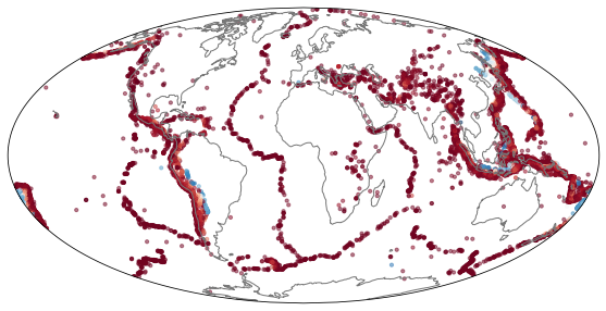
Define a relatively smooth function that we can interpolate from the coarse mesh to the fine mesh and analyse. As it is a familiar pattern, we use the seismic event catalogue for M5.5+ (dawn of time to 2017-12-31) from IRIS
import numpy as np

# Note - these data have some places where depth is unknown (appears as NaN in the depth )
# The IRIS data has  lat, lon, depth, mag  ... date/time in col 2, 3, 4, 10 (starting from zero)

eqs = np.genfromtxt("../Data/EQ-M5.5-IRIS-ALL.txt", usecols=(2,3,4,10), delimiter='|', comments="#")


lons = np.radians(eqs[:,1])
lats = np.radians(eqs[:,0])
depths = eqs[:,2]
depths[np.isnan(depths)] = -1.0
%matplotlib inline

import cartopy
import cartopy.crs as ccrs
import matplotlib.pyplot as plt

fig = plt.figure(figsize=(10, 5), facecolor="none")
ax  = plt.subplot(111, projection=ccrs.Mollweide())
ax.coastlines(color="#777777" )
ax.set_global()

lons0 = np.degrees(lons)
lats0 = np.degrees(lats)

ax.scatter(lons0, lats0,
            marker="o", s=10.0, alpha=0.5,
            transform=ccrs.PlateCarree(), c=depths, cmap=plt.cm.RdBu)

pass
Count earthquakes per triangle
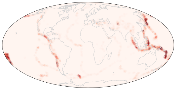
This is a numpy wrapper around the STRIPACK routine which operates by retriangulation and is therefore not particularly fast.
triangles = mesh.containing_triangle(lons, lats)
## The return_counts argument is quite new in numpy and your version may not have it

try:
    tris, counts = np.unique(triangles, return_counts=True)
except:

    def unique_count(a):
        unique, inverse = np.unique(a, return_inverse=True)
        count = np.zeros(len(unique), np.int)
        np.add.at(count, inverse, 1)
        return unique, count

    tris, counts = unique_count(triangles)
tris.shape
(3382,)
## map to nodes so we can plot this

hit_count = np.zeros_like(mesh.lons)

for i in range(0, tris.shape[0]):
    hit_count[mesh.simplices[tris[i]]] += counts[i]

hit_count /= 3.0

print(hit_count.mean())
0.42119653668380963
fig = plt.figure(figsize=(10, 10), facecolor="none")
ax  = plt.subplot(111, projection=ccrs.Mollweide())
ax.coastlines(color="lightgrey", )
ax.set_global()

lons0 = np.degrees(mesh.lons)
lats0 = np.degrees(mesh.lats)

ax.scatter(lons0, lats0,
            marker="o", s=30.0, transform=ccrs.PlateCarree(), c=hit_count, cmap=plt.cm.Reds, vmin=0.333, vmax=20.0, alpha=0.25)

pass
Count earthquakes per vertex
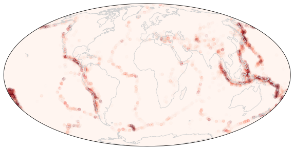
The sTriangulation.nearest_vertices method uses a k-d tree to find the nearest vertices to a set of longitude / latitude points. It returns the great circle distance. This requires the k-d tree to have been built when the mesh was initialised (tree=True)
distances, vertices = mesh.nearest_vertices(lons, lats, k=1)
nodes, ncounts = np.unique(vertices, return_counts=True)

hit_countn = np.zeros_like(mesh.lons)
hit_countn[nodes] = ncounts
fig = plt.figure(figsize=(10, 10), facecolor="none")
ax  = plt.subplot(111, projection=ccrs.Mollweide())
ax.coastlines(color="lightgrey", )
ax.set_global()

lons0 = np.degrees(mesh.lons)
lats0 = np.degrees(mesh.lats)

ax.scatter(lons0, lats0,
            marker="o", s=30.0, transform=ccrs.PlateCarree(), c=hit_countn, cmap=plt.cm.Reds, vmin=0.333, vmax=10.0, alpha=0.25)

pass
Inverse distance weighted number of earthquakes
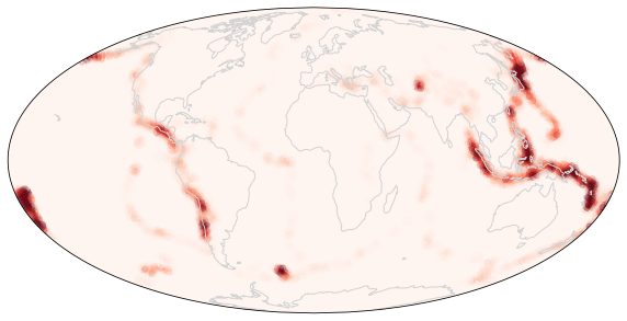
The k-d tree method provides a specified number of neighbours and the arc lengths to those neighbours. This can be used in a number of ways to smooth or amalgamate data. Here for example is a weighted average of each earthquake to nearby nodes.
We compute the distances to \(N\) nearby vertices and distribute information to those vertices in inverse proportion to their distance.
Alternatively, we might map information to the vertices by applying a radially symmetric kernel to the point data without normalising.
distances, vertices = mesh.nearest_vertices(lons, lats, k=10)
norm = distances.sum(axis=1)

# distances, vertices are arrays of shape (data_size, 10)

hit_countid = np.zeros_like(mesh.lons)

## numpy shouldn't try to vectorise this reduction operation

for i in range(0,distances.shape[0]):
    hit_countid[vertices[i,:]] += distances[i,:] / norm[i]


hit_countidr = np.zeros_like(mesh.lons)

## numpy shouldn't try to vectorise this reduction operation

for i in range(0,distances.shape[0]):
    hit_countidr[vertices[i,:]] += np.exp( -distances[i,:] / 0.02 )
fig = plt.figure(figsize=(10, 10), facecolor="none")
ax  = plt.subplot(111, projection=ccrs.Mollweide())
ax.coastlines(color="lightgrey", )
ax.set_global()

lons0 = np.degrees(mesh.lons)
lats0 = np.degrees(mesh.lats)

ax.scatter(lons0, lats0,
            marker="o", s=30.0, transform=ccrs.PlateCarree(), c=hit_countid, cmap=plt.cm.Reds, vmin=0.333, vmax=10.0, alpha=0.25)

pass
Mapping data other than frequency to the regular mesh
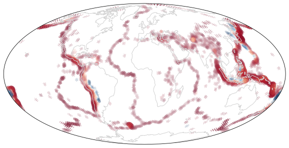
Here we show how to map point data to the regular mesh - produce a representation of the depth of the events instead of just their frequency. When plotting, we need to distinguish between zero information and zero (shallow) depth. This is done by using the weight function to determine the opacity of the symbol or field that we plot. This has the effect of washing out the regions with few, large events compared to those with many small ones (which in this case means washed out regions where earthquakes are deep).
depth_idr = np.zeros_like(mesh.lons)

## numpy shouldn't try to vectorise this reduction operation

for i in range(0,distances.shape[0]):
    depth_idr[vertices[i,:]] += depths[i] * np.exp( -distances[i,:] / 0.02 )

depth_idr[hit_countidr != 0.0] /=  hit_countidr[hit_countidr != 0.0]
fig = plt.figure(figsize=(10, 10), facecolor="none")
ax  = plt.subplot(111, projection=ccrs.Mollweide())
ax.coastlines(color="lightgrey", )
ax.set_global()

lons0 = np.degrees(mesh.lons)
lats0 = np.degrees(mesh.lats)

ax.scatter(lons0, lats0,
            marker="o", transform=ccrs.PlateCarree(), c=depth_idr, s=hit_countidr,
            cmap=plt.cm.RdBu, vmin=0.0, vmax=500.0, alpha=0.25)

pass
Visualisation
import k3d

plot = k3d.plot(camera_auto_fit=False, grid_visible=False,
                menu_visibility=True, axes_helper=False )

indices = mesh.simplices.astype(np.uint32)
points = np.column_stack(mesh.points.T).astype(np.float32)

mesh_viewer = k3d.mesh(points, indices, wireframe=False, attribute=hit_count,
                   color_map=k3d.colormaps.paraview_color_maps.Cool_to_Warm,
                   name="heat map",
                   flat_shading=False, opacity=1.0  )

## This helps to manage the wireframe / transparency
background = k3d.mesh(points*0.95, indices, wireframe=False,
                   color=0xBBBBBB, opacity=1.0, flat_shading=False  )


plot   += mesh_viewer
plot += background
plot.display()

## ## ##

from ipywidgets import interact, interactive
import ipywidgets as widgets

choices = { "hit_count": hit_count,
             "hit_countn": hit_countn,
             "hit_countid": hit_countid,
             "hit_countidr": hit_countidr,
             "depth_idr": depth_idr  }

@interact(choice=choices.keys())
def chooser(choice):
    mesh_viewer.attribute = choices[choice].astype(np.float32)
    range = choices[choice].max() * 0.2
    mesh_viewer.color_range = [0, range]
    return
The next example is Ex7-Refinement-of-Triangulations