Tutorials
Underworld is designed to be run in the jupyter notebook environment where you can take advantage of jupyter’s rich display capabilities to explore the mathematics of your problem, visualise results and query classes or live objects.
You will find it helpful for developing scripts and analysing results. If you use jupytext to write notebooks directly as python scripts, then the same notebook codes will run on a parallel machine with no performance penalty.
The notebooks are rendered as html pages in this guide. They are distributed with the source code on GitHub and can be run on binder.
Notebook 1 - Meshes
Meshes: Introduces the mesh discretisation that we use in Underworld3 and how you can build one of the pre-defined meshes. This notebook also show you how to use the pyvista visualisation tools for Underworld3 objects. The mesh holds information on the mesh geometry, boundaries and coordinate systems.
Notebook 2 - Mesh Variables
Variables: Introduces the concept of MeshVariables in Underworld3. These are both data containers and sympy symbolic objects. We show you how to inspect a meshVariable, set the data values in the MeshVariable and visualise them.
Notebook 3 - Symbols and sympy
Symbols: meshVariables are sympy objects that can be composed with other symbolic objects and evaluated numerically when required. They can also be differentiated. Most importantly, sympy can manipulate expressions, simplify them and cancel terms.
Notebook 4 - Example: Diffusion Equation
Diffusion Solver: Introduces the various solver templates that are available in Underworld, starting with a steady-state diffusion problem. The template requires you to set some constitutive properties and define the unknowns. These are handled through subsitution into symbolic forms and the template equation can be inspected before you need to supply concrete expressions.
Notebook 5 - Example: Stokes Equation
Stokes Solver: Stokes equation is a more complicated system of equations to solve. This complexity is mostly hidden when you set the problem up. There are some interesting ways to constrain boundary values which are demonstrated using an annulus mesh (curved, free-slip boundaries) and a \(\delta\) function buoyancy source.
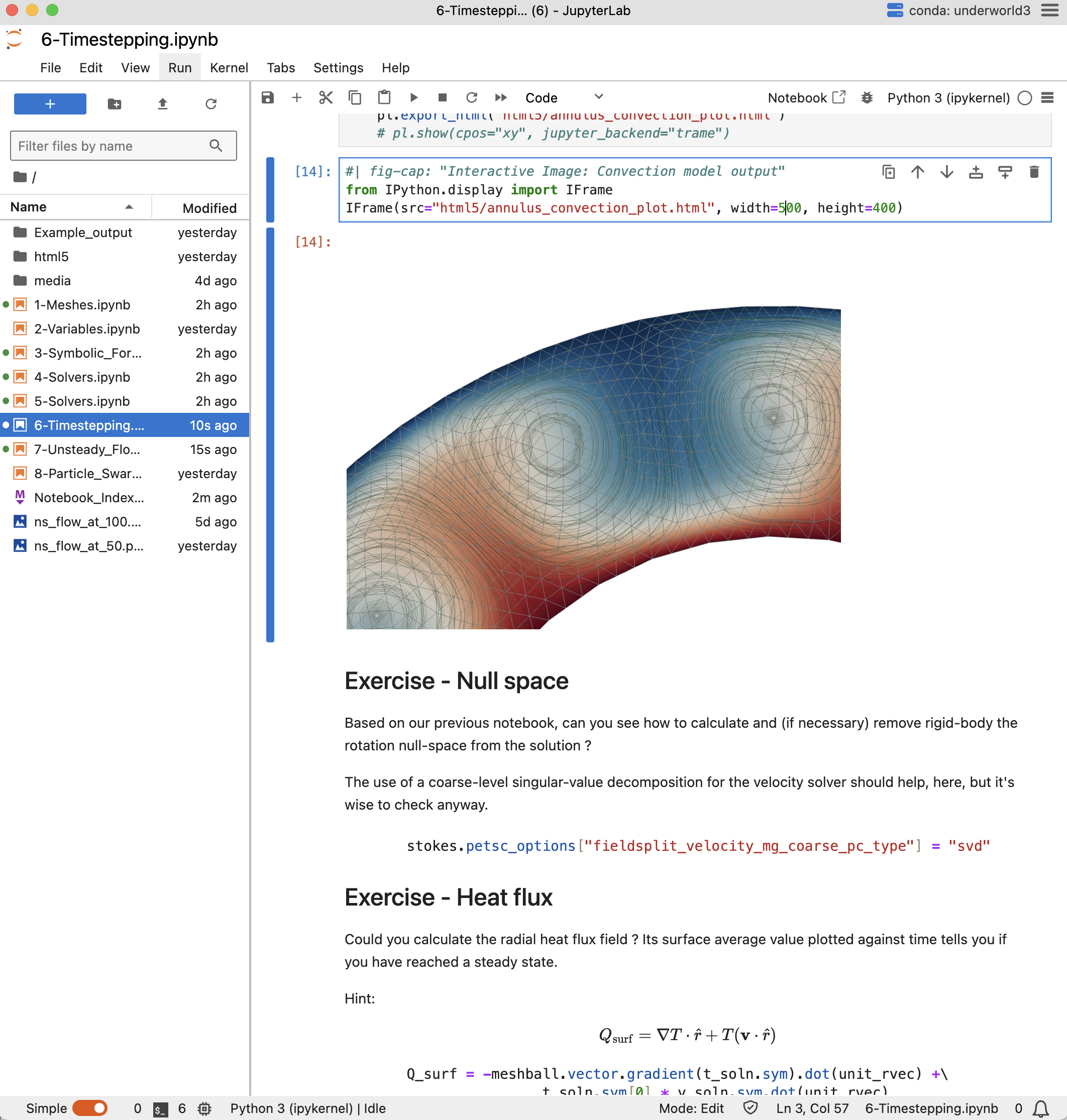
Notebook 6 - Example: Time Dependence
Timestepping: Coupled Stokes flow plus thermal advection-diffusion gives a simple convection solver. The timestepping loop is written by hand because usually you will want to do some analysis or output some checkpoints.
Notebook 8 - Lagrangian Swarm Variables
Swarm Variables - exploring how they work for specifying material properties with a swarm used to determine element viscosity. We learn how to use swarm variables in expressions generally and for boundary conditions.