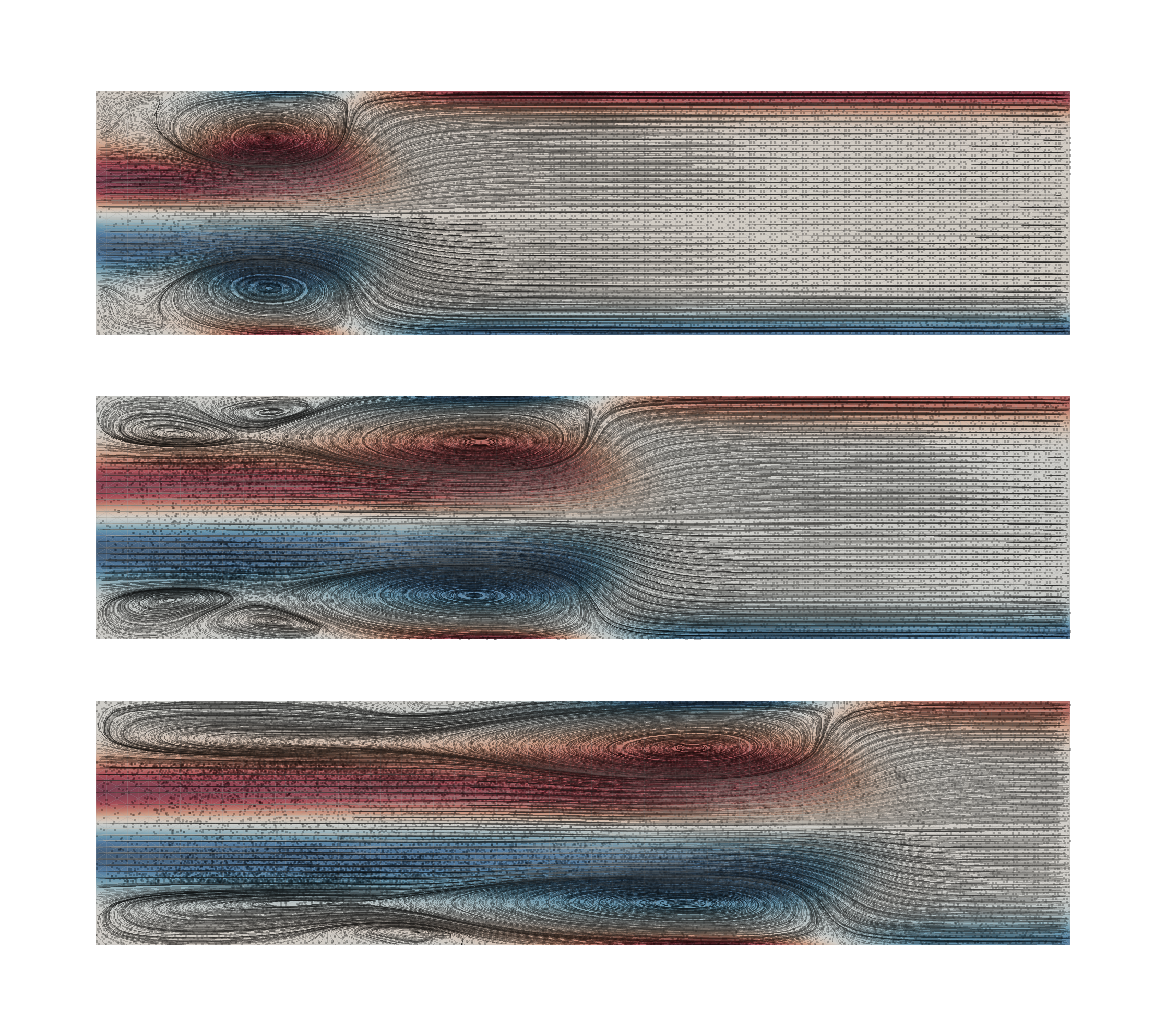
Flow in a pipe with inflow at the left boundary after 50, 100, 150 timesteps (top to bottom) showing the progression of the impulsive initial condition. For details, see the notebook code.
We’ll look at tracking an unsteady flow using a swarm of particle flow-tracers. In this case, the flow is unsteady because we solve the Navier-Stokes equation (that is, the flow has inertia) and we impose an impulsive, initial boundary velocity.
To begin with, the set up follows the same path as all previous notebooks: - Create a mesh - Add some variables - Create the solver we need (NavierStokes this time) - Add boundary conditions and constitutive properties.
We also add a projection solver to compute the vorticity of the flow as we did in Notebook 4 when we needed to compute a heat-flux (thermal gradient) term.
To track the time evolution of the flow, we introduce a “passive” particle swarm. Passive, here, refers to the fact that the flow is not changed by the presence of the marker particles.
In the time-loop we have to update the particle locations and we keep this as an explicity operation, in general, because it provide the opportunity for you to make changes or perform analyses. In this case, we are adding new particles near the inflow to track the flow.
To learn more about flow goverened by the Navier-Stokes equation, it may be he helpful to read an elementary fluid dynamics textbook and reproduce some of the simple “toy” examples. For example, Acheson, 1990.
import numpy as npimport sympyimport underworld3 as uw
res =8width =4reynolds_number =1000mesh = uw.meshing.UnstructuredSimplexBox( cellSize=1/ res, minCoords=(0.0, 0.0), maxCoords=(width, 1.0), qdegree=3,)# Coordinate directions etcx, y = mesh.CoordinateSystem.X
The Navier-Stokes solver is a combination of a Stokes solver with time-dependent terms for both the Flux history and velocity history. These are orchestrated behind the scenes but some user-accessible options can be set, and full introspection is available using the view methods.
The velocity history terms are implemented using uw.systems.ddt objects (Eulerian, Semi-Lagrangian (default), or Lagrangian). Use navier_stokes.DFDt.view(class_documentation=True) and navier_stokes.DuDt.view(class_documentation=True) for more information.
The ddt objects implement the Adams-Moulton schemes for flux-terms (order=1 implemented the well-known Crank-Nicholson scheme). For the velocity history term, backward differentiation formulae are used. Introspection for the NS solver shows how the various terms combine to form the full set of equations.
uw.systems.NavierStokes.view()
Navier-Stokes Equation Solver
This class provides a solver for the Navier-Stokes (vector Advection-Diffusion) equation which is similar to that used in the Semi-Lagrange Crank-Nicholson method (Spiegelman & Katz, 2006) but using a distributed sampling of upstream values taken from an arbitrary swarm variable.
The term \(\mathbf{F}\) relates diffusive fluxes to gradients in the unknown \(u\). The advective flux that results from having gradients along the direction of transport (given by the velocity vector field \(\mathbf{v}\) ) are included in the \(\dot{\mathbf{u}}\) term.
The term \(\dot{\mathbf{u}}\) involves upstream sampling to find the value \(u^{ * }\) which represents the value of \(u\) at the beginning of the timestep. This is achieved using a swarmVariable that carries history information along the flow path. A dense sampling is required to achieve similar accuracy to the original SLCN approach but it allows the use of a single swarm for history tracking of variables with different interpolation order and for material tracking. The user is required to supply and update the swarmVariable representing \(u^{ * }\)
Properties
The unknown is \(u\).
The history variable is \(u^*\) and is provided in the form of a sympy function. It is the user’s responsibility to keep this variable updated.
The diffusivity tensor, \(\kappa\) is provided by setting the constitutive_model property to one of the scalar uw.constitutive_models classes and populating the parameters. It is usually a constant or a function of position / time and may also be non-linear or anisotropic.
Volumetric sources of \(u\) are specified using the \(f\) property and can be any valid combination of sympy functions of position and meshVariable or swarmVariable types.
Notes
The solver requires relatively high order shape functions to accurately interpolate the history terms. Spiegelman & Katz recommend cubic or higher degree for \(u\) but this is not checked.
References
Spiegelman, M., & Katz, R. F. (2006). A semi-Lagrangian Crank-Nicolson algorithm for the numerical solution of advection-diffusion problems. Geochemistry, Geophysics, Geosystems, 7(4). https://doi.org/10.1029/2005GC001073
navier_stokes.DuDt.view(class_documentation=True)
Nodal-Swarm Semi-Lagrangian History Manager:
This manages the semi-Lagrangian update of a Mesh Variable, \(\psi\), on the mesh across timesteps. \[\quad \psi_p^{t-n\Delta t} \leftarrow \psi_p^{t-(n-1)\Delta t}\quad\]\[\quad \psi_p^{t-(n-1)\Delta t} \leftarrow \psi_p^{t-(n-2)\Delta t} \cdots\quad\]\[\quad \psi_p^{t-\Delta t} \leftarrow \psi_p^{t}\]
# Keep the initialisation separate# so we can run the loop below again without resetting# the timer.max_steps =50timestep =0elapsed_time =0.0delta_t =0.05
for step inrange(0, max_steps):# Keep previous guess for solve navier_stokes.solve(zero_init_guess=False, timestep=delta_t) passive_swarm.advection(v_soln.sym, delta_t, order=2, corrector=False)# Add new tracer particles near the inlet new_points =100 new_coords = np.array([0.0, 0.25] +0.5* np.random.random((new_points, 2))) passive_swarm.add_particles_with_coordinates(new_coords)# Save the data at every 10th stepif timestep %10==0: vorticity_from_v.solve() mesh.write_timestep("Example_7", meshUpdates=True, meshVars=[p_soln, v_soln, vorticity], outputPath="Example_output", index=timestep, ) passive_swarm.write_timestep("Example_7","passive_swarm", swarmVars=None, outputPath="Example_output", index=timestep, force_sequential=True, ) timestep +=1 elapsed_time += delta_tprint(f"Timestep: {timestep}, time {elapsed_time:.4f}")
Timestep: 1, time 0.0500
Timestep: 2, time 0.1000
Timestep: 3, time 0.1500
Timestep: 4, time 0.2000
Timestep: 5, time 0.2500
Timestep: 6, time 0.3000
from IPython.display import IFrameIFrame(src=f"html5/ns_flow_plot_50.html", width=1000, height=400)
Interactive Image: Time-dependent model output
Exercise - 7.1
Now that you have seen the structure of the flow in this example, can you adjust the addition of particles to capture the structure more clearly ?
This is a very low-resolution example. You can try increasing the resolution but you will see that this would benefit from running in parallel. In parallel we should remove all the visualisation and visualise the h5 output files when we are done. The rest of the code is parallel-safe.
References
Acheson, D. J. (1990). Elementary Fluid Dynamics. Oxford University PressOxford. https://doi.org/10.1093/oso/9780198596608.001.0001