import numpy as np
import sympy
import underworld3 as uwNotebook 6: Rayleigh-Bénard Convection (time-stepping example)
We’ll look at a convection problem which couples Stokes Flow with time-dependent advection/diffusion to give simple Rayleigh-Bénard convection model.
\[ -\nabla \cdot \left[ \frac{\eta}{2}\left( \nabla \mathbf{u} + \nabla \mathbf{u}^T \right) - p \mathbf{I} \right] = -\rho_0 \alpha T \mathbf{g} \] \[ \nabla \cdot \mathbf{u} = 0 \]
\(\eta\) is viscosity, \(p\) is pressure, \(\rho_0\) is a reference density, \(\alpha\) is thermal expansivity, and \(T\) is the temperature. Here we explicitly express density variations in terms of temperature variations.
Thermal evolution is given by \[ \frac{\partial T}{\partial t} - \mathbf{u}\cdot\nabla T = \kappa \nabla^2 T \] where the velocity, \(\mathbf{u}\) is the result of the Stokes flow calculation. \(\kappa\) is the thermal diffusivity (compare this with Notebook 4).
The starting point is our previous notebook where we solved for Stokes flow in a cylindrical annulus geometry. We then add an advection-diffusion solver to evolve temperature. The Stokes buoyancy force is proportional to the temperature anomaly, and the velocity solution is fed back into the temperature advection term. The timestepping loop is written by hand because usually you will want to do some analysis or output some checkpoints.
To read more about the applications of simple mantle convection models like this one, see (for example) Schubert et al, 2001.
res = 10
r_o = 1.0
r_i = 0.55

rayleigh_number = 3.0e4

meshball = uw.meshing.Annulus(
    radiusOuter=r_o,
    radiusInner=r_i,
    cellSize=1 / res,
    qdegree=3,
)

# Coordinate directions etc
x, y = meshball.CoordinateSystem.X
r, th = meshball.CoordinateSystem.xR
unit_rvec = meshball.CoordinateSystem.unit_e_0

# Orientation of surface normals
Gamma_N = unit_rvec
# Mesh variables for the unknowns
v_soln = uw.discretisation.MeshVariable("V0", meshball, 2, degree=2, varsymbol=r"{v_0}")
p_soln = uw.discretisation.MeshVariable("p", meshball, 1, degree=1, continuous=True)
t_soln = uw.discretisation.MeshVariable("T", meshball, 1, degree=3, continuous=True)Create linked solvers
We create the Stokes solver as we did in the previous notebook. The buoyancy force is proportional to the temperature anomaly (t_soln). Solvers can either be provided with unknowns as pre-defined meshVariables, or they will define their own. When solvers are coupled, explicitly defining unknowns makes everything clearer.
The advection-diffusion solver evolved t_soln using the Stokes velocity v_soln in the fluid-transport term.
Curved, free-slip boundaries
In the annulus, a free slip boundary corresponds to zero radial velocity. However, in this mesh, \(v_r\) is not one of the unknowns (\(\mathbf{v} = (v_x, v_y)\)). We apply a non linear boundary condition that penalises \(v_r\) on the boundary as discussed previously in Example 5.
stokes = uw.systems.Stokes(
    meshball,
    velocityField=v_soln,
    pressureField=p_soln,
)

stokes.bodyforce = rayleigh_number * t_soln.sym * unit_rvec

stokes.constitutive_model = uw.constitutive_models.ViscousFlowModel
stokes.constitutive_model.Parameters.shear_viscosity_0 = 1
stokes.tolerance = 1.0e-3

stokes.petsc_options["fieldsplit_velocity_mg_coarse_pc_type"] = "svd"

stokes.add_natural_bc(1000000 * Gamma_N.dot(v_soln.sym) * Gamma_N, "Upper")

if r_i != 0.0:
    stokes.add_natural_bc(1000000 * Gamma_N.dot(v_soln.sym) * Gamma_N, "Lower")
# Create solver for the energy equation (Advection-Diffusion of temperature)
adv_diff = uw.systems.AdvDiffusion(
meshball,
u_Field=t_soln,
V_fn=v_soln,
order=2,
verbose=False,
)
adv_diff.constitutive_model = uw.constitutive_models.DiffusionModel
adv_diff.constitutive_model.Parameters.diffusivity = 1
## Boundary conditions for this solver
adv_diff.add_dirichlet_bc(+1.0, "Lower")
adv_diff.add_dirichlet_bc(-0.0, "Upper")
adv_diff.petsc_options.setValue("snes_rtol", 0.001)
adv_diff.petsc_options.setValue("ksp_rtol", 0.0001)
adv_diff.petsc_options.setValue("snes_monitor", None)
adv_diff.petsc_options.setValue("ksp_monitor", None)uw.systems.AdvDiffusion.view()Advection-Diffusion Equation Solver (Scalar Variable)
This class provides a solver for the scalar Advection-Diffusion equation using the characteristics based Semi-Lagrange Crank-Nicholson method which is described in Spiegelman & Katz, (2006).
\[ \color{Green}{\underbrace{ \Bigl[ \frac{\partial u}{\partial t} + \left( \mathbf{v} \cdot \nabla \right) u \Bigr]}_{\dot{\mathbf{u}}}} - \nabla \cdot \color{Blue}{\underbrace{\Bigl[ \boldsymbol\kappa \nabla u \Bigr]}_{\mathbf{F}}} = \color{Maroon}{\underbrace{\Bigl[ f \Bigl] }_{\mathbf{h}}} \]
The term \(\mathbf{F}\) relates diffusive fluxes to gradients in the unknown \(u\). The advective flux that results from having gradients along the direction of transport (given by the velocity vector field \(\mathbf{v}\) ) are included in the \(\dot{\mathbf{u}}\) term.
The term \(\dot{\mathbf{u}}\) involves upstream sampling to find the value \(u^*\) which represents the value of \(u\) at the points which later arrive at the nodal points of the mesh. This is achieved using a “hidden” swarm variable which is advected backwards from the nodal points automatically during the solve phase.
Properties
The unknown is \(u\).
The velocity field is \(\mathbf{v}\) and is provided as a
sympyfunction to allow operations such as time-averaging to be calculated in situ (e.g.V_Field = v_solution.sym) NOTE: no it’s not. Currently it is a MeshVariable this is the desired behaviour though.The diffusivity tensor, \(\kappa\) is provided by setting the
constitutive_modelproperty to one of the scalaruw.constitutive_modelsclasses and populating the parameters. It is usually a constant or a function of position / time and may also be non-linear or anisotropic.Volumetric sources of \(u\) are specified using the \(f\) property and can be any valid combination of
sympyfunctions of position andmeshVariableorswarmVariabletypes.
References
Spiegelman, M., & Katz, R. F. (2006). A semi-Lagrangian Crank-Nicolson algorithm for the numerical solution of advection-diffusion problems. Geochemistry, Geophysics, Geosystems, 7(4). https://doi.org/10.1029/2005GC001073
uw.systems.SemiLagragian_DDt.view()Nodal-Swarm Lagrangian History Manager: This manages the update of a Lagrangian variable, \(\psi\) on the swarm across timesteps. \[\quad \psi_p^{t-n\Delta t} \leftarrow \psi_p^{t-(n-1)\Delta t}\quad\] \[\quad \psi_p^{t-(n-1)\Delta t} \leftarrow \psi_p^{t-(n-2)\Delta t} \cdots\quad\] \[\quad \psi_p^{t-\Delta t} \leftarrow \psi_p^{t}\]
Underworld expressions
Note that the parameters in the consititutive models are defined as uw.expressions because 1. We generally would like to display them symbolically in equations rather than see their floating point value 2. They can represent complex expressions that “blow up” the symbolic forms when we inspect the equations 3. We would like to be able to substitute new values in the equations and use the lazy evaluation of expressions to avoid having to redefine expressions in multiple locations where these symbols appear 4. For future reference, in optimisation problems, we differentiate expressions with respect to their parameters and want the results also to be evaluated in a lazy fashion.
display(type(stokes.constitutive_model.Parameters.shear_viscosity_0))
display(type(adv_diff.constitutive_model.Parameters.diffusivity))

stokes.constitutive_model.Parameters.shear_viscosity_0.symunderworld3.function.expressions.UWexpressionunderworld3.function.expressions.UWexpression\(\displaystyle 1\)
Initial condition
We need to set an initial condition for the temperature field as the coupled system is an initial value problem. Choose whatever works but remember that the boundary conditions will over-rule values you set on the lower and upper boundaries.
# Initial temperature

init_t = 0.1 * sympy.sin(3 * th) * sympy.cos(np.pi * (r - r_i) / (r_o - r_i)) + (
    r_o - r
) / (r_o - r_i)

with meshball.access(t_soln):
    t_soln.data[:, 0] = uw.function.evaluate(init_t, t_soln.coords)
Initial velocity solve
The first solve allows us to determine the magnitude of the velocity field and is useful to keep separated to check convergence rates etc.
For non-linear problems, we usually need an initial guess using a reasonably close linear problem.
zero_init_guess is used to reset any information in the vector of unknowns (i.e. do not use any initial information if zero_init_guess==True).
stokes.solve(zero_init_guess=True)# Keep the initialisation separate
# so we can run the loop again in a notebook
max_steps = 15
timestep = 0
elapsed_time = 0.0adv_diff.view(class_documentation=True)Advection-Diffusion Equation Solver (Scalar Variable)
This class provides a solver for the scalar Advection-Diffusion equation using the characteristics based Semi-Lagrange Crank-Nicholson method which is described in Spiegelman & Katz, (2006).
\[ \color{Green}{\underbrace{ \Bigl[ \frac{\partial u}{\partial t} + \left( \mathbf{v} \cdot \nabla \right) u \Bigr]}_{\dot{\mathbf{u}}}} - \nabla \cdot \color{Blue}{\underbrace{\Bigl[ \boldsymbol\kappa \nabla u \Bigr]}_{\mathbf{F}}} = \color{Maroon}{\underbrace{\Bigl[ f \Bigl] }_{\mathbf{h}}} \]
The term \(\mathbf{F}\) relates diffusive fluxes to gradients in the unknown \(u\). The advective flux that results from having gradients along the direction of transport (given by the velocity vector field \(\mathbf{v}\) ) are included in the \(\dot{\mathbf{u}}\) term.
The term \(\dot{\mathbf{u}}\) involves upstream sampling to find the value \(u^*\) which represents the value of \(u\) at the points which later arrive at the nodal points of the mesh. This is achieved using a “hidden” swarm variable which is advected backwards from the nodal points automatically during the solve phase.
Properties
The unknown is \(u\).
The velocity field is \(\mathbf{v}\) and is provided as a
sympyfunction to allow operations such as time-averaging to be calculated in situ (e.g.V_Field = v_solution.sym) NOTE: no it’s not. Currently it is a MeshVariable this is the desired behaviour though.The diffusivity tensor, \(\kappa\) is provided by setting the
constitutive_modelproperty to one of the scalaruw.constitutive_modelsclasses and populating the parameters. It is usually a constant or a function of position / time and may also be non-linear or anisotropic.Volumetric sources of \(u\) are specified using the \(f\) property and can be any valid combination of
sympyfunctions of position andmeshVariableorswarmVariabletypes.
References
Spiegelman, M., & Katz, R. F. (2006). A semi-Lagrangian Crank-Nicolson algorithm for the numerical solution of advection-diffusion problems. Geochemistry, Geophysics, Geosystems, 7(4). https://doi.org/10.1029/2005GC001073
Class: <class ‘underworld3.systems.solvers.SNES_AdvectionDiffusion’>
Underworld / PETSc General Scalar Equation Solver
Primary problem:
<IPython.core.display.Latex object>$ = 0 $
Where:
\(\quad\)\(\displaystyle \upkappa\)\(=\)\(\displaystyle 1\)
\(\quad\)\(\displaystyle \Delta t\)\(=\)\(\displaystyle 0.00192729179220545\)
Boundary Conditions
| Type | Boundary | Expression |
|---|---|---|
| essential | Lower | $$ |
| essential | Upper | $$ |
This solver is formulated as a 2 dimensional problem with a 2 dimensional mesh
$ = $ \(\displaystyle \left[\begin{matrix}{ \hspace{ 0.04pt } {T} }(\mathbf{x})\end{matrix}\right]\)
$ = $ \(\displaystyle \left[\begin{matrix}{ \hspace{ 0.04pt } {{v_0}} }_{ 0 }(\mathbf{x}) & { \hspace{ 0.04pt } {{v_0}} }_{ 1 }(\mathbf{x})\end{matrix}\right]\)
$t = $ \(\displaystyle \Delta t\)
init_t = 0.1 * sympy.sin(3 * th) * sympy.cos(np.pi * (r - r_i) / (r_o - r_i)) + (
    r_o - r
) / (r_o - r_i)

with meshball.access(t_soln):
    t_soln.data[:, 0] = uw.function.evaluate(
        init_t + 0.0001 * t_soln.sym[0], adv_diff.DuDt.psi_star[0].coords
)adv_diff.estimate_dt()0.0015310756944410533adv_diff.solve(timestep=0.01, zero_init_guess=True) 0 SNES Function norm 9.477337251545e+00
Residual norms for Solver_14_ solve.
0 KSP Residual norm 5.145688853471e+01
1 KSP Residual norm 6.664452877949e+00
2 KSP Residual norm 1.519834146720e+00
3 KSP Residual norm 8.840183259526e-01
4 KSP Residual norm 5.301397793504e-01
5 KSP Residual norm 2.424966321832e-01
6 KSP Residual norm 1.150826566498e-01
7 KSP Residual norm 6.172825406475e-02
8 KSP Residual norm 3.137375512549e-02
9 KSP Residual norm 1.401218686048e-02
10 KSP Residual norm 6.780473869117e-03
11 KSP Residual norm 3.790531875925e-03
1 SNES Function norm 3.383398820327e-03# Null space ?
for step in range(0, max_steps):
stokes.solve(zero_init_guess=False)
delta_t = 5 * adv_diff.estimate_dt()
adv_diff.solve(timestep=delta_t, zero_init_guess=False, verbose=False)
timestep += 1
elapsed_time += delta_t
if timestep % 5 == 0:
print(f"Timestep: {timestep}, time {elapsed_time}") 0 SNES Function norm 5.519719545520e-01
Residual norms for Solver_14_ solve.
0 KSP Residual norm 1.080481897680e+00
1 KSP Residual norm 2.794759495722e-01
2 KSP Residual norm 8.738937475137e-02
3 KSP Residual norm 2.538497096191e-02
4 KSP Residual norm 9.791736400409e-03
5 KSP Residual norm 3.712676600336e-03
6 KSP Residual norm 1.063757340521e-03
7 KSP Residual norm 4.172823722413e-04
8 KSP Residual norm 1.562544824097e-04
9 KSP Residual norm 5.223214632822e-05
1 SNES Function norm 4.882999045393e-05
0 SNES Function norm 4.773557354896e-01
Residual norms for Solver_14_ solve.
0 KSP Residual norm 9.317588273285e-01
1 KSP Residual norm 2.459336490176e-01
2 KSP Residual norm 7.783642668213e-02
3 KSP Residual norm 2.191611878110e-02
4 KSP Residual norm 6.968378956074e-03
5 KSP Residual norm 3.165364530306e-03
6 KSP Residual norm 1.009565335997e-03
7 KSP Residual norm 4.012564067190e-04
8 KSP Residual norm 1.480223863671e-04
9 KSP Residual norm 5.045767013406e-05
1 SNES Function norm 4.665072060480e-05
0 SNES Function norm 4.134346531441e-01
Residual norms for Solver_14_ solve.
0 KSP Residual norm 8.307659270725e-01
1 KSP Residual norm 2.259694308441e-01
2 KSP Residual norm 6.843626200604e-02
3 KSP Residual norm 2.044900509918e-02
4 KSP Residual norm 7.902904914890e-03
5 KSP Residual norm 3.123583935771e-03
6 KSP Residual norm 9.710014509369e-04
7 KSP Residual norm 4.067866782756e-04
8 KSP Residual norm 1.440315988629e-04
9 KSP Residual norm 4.828499765245e-05
1 SNES Function norm 4.388299556922e-05
0 SNES Function norm 3.702917051432e-01
Residual norms for Solver_14_ solve.
0 KSP Residual norm 7.391018432834e-01
1 KSP Residual norm 2.118225742668e-01
2 KSP Residual norm 6.153300528419e-02
3 KSP Residual norm 1.888671986332e-02
4 KSP Residual norm 7.688485116852e-03
5 KSP Residual norm 2.892614443447e-03
6 KSP Residual norm 9.899961279690e-04
7 KSP Residual norm 4.303831257914e-04
8 KSP Residual norm 1.400355896622e-04
9 KSP Residual norm 4.622207543067e-05
1 SNES Function norm 4.202452224287e-05
0 SNES Function norm 3.315890905574e-01
Residual norms for Solver_14_ solve.
0 KSP Residual norm 6.598577757155e-01
1 KSP Residual norm 1.933887338875e-01
2 KSP Residual norm 5.456342813682e-02
3 KSP Residual norm 1.650324248410e-02
4 KSP Residual norm 6.568305659431e-03
5 KSP Residual norm 2.510214143805e-03
6 KSP Residual norm 8.758541569735e-04
7 KSP Residual norm 3.932827467617e-04
8 KSP Residual norm 1.269075769185e-04
9 KSP Residual norm 4.140260482029e-05
1 SNES Function norm 3.796231562527e-05
Timestep: 35, time 0.11813280083141166
0 SNES Function norm 2.960859596617e-01
Residual norms for Solver_14_ solve.
0 KSP Residual norm 5.869188962370e-01
1 KSP Residual norm 1.726402385232e-01
2 KSP Residual norm 4.810609894045e-02
3 KSP Residual norm 1.599606132489e-02
4 KSP Residual norm 6.662165427614e-03
5 KSP Residual norm 2.357922152146e-03
6 KSP Residual norm 8.726421811308e-04
7 KSP Residual norm 3.684349989627e-04
8 KSP Residual norm 1.156301902495e-04
9 KSP Residual norm 3.679909417202e-05
1 SNES Function norm 3.370864114565e-05
0 SNES Function norm 2.635627796534e-01
Residual norms for Solver_14_ solve.
0 KSP Residual norm 5.258120790880e-01
1 KSP Residual norm 1.546764180521e-01
2 KSP Residual norm 4.243034265403e-02
3 KSP Residual norm 1.387021411069e-02
4 KSP Residual norm 5.708313168922e-03
5 KSP Residual norm 2.062686684951e-03
6 KSP Residual norm 7.701770867568e-04
7 KSP Residual norm 3.260237474077e-04
8 KSP Residual norm 1.016927787321e-04
9 KSP Residual norm 3.305441847160e-05
1 SNES Function norm 3.021711111259e-05
0 SNES Function norm 2.352577982225e-01
Residual norms for Solver_14_ solve.
0 KSP Residual norm 4.662224909913e-01
1 KSP Residual norm 1.308304571920e-01
2 KSP Residual norm 3.675067184174e-02
3 KSP Residual norm 1.198851986901e-02
4 KSP Residual norm 4.847809939836e-03
5 KSP Residual norm 1.779671490862e-03
6 KSP Residual norm 6.606400480385e-04
7 KSP Residual norm 2.862974583735e-04
8 KSP Residual norm 9.092912549642e-05
9 KSP Residual norm 2.899026967379e-05
1 SNES Function norm 2.618219715153e-05
0 SNES Function norm 2.081588556650e-01
Residual norms for Solver_14_ solve.
0 KSP Residual norm 4.156850990805e-01
1 KSP Residual norm 1.156419232977e-01
2 KSP Residual norm 3.377209422854e-02
3 KSP Residual norm 1.082700216683e-02
4 KSP Residual norm 4.371252675824e-03
5 KSP Residual norm 1.608015818152e-03
6 KSP Residual norm 5.939159194124e-04
7 KSP Residual norm 2.567259407852e-04
8 KSP Residual norm 8.090958515797e-05
9 KSP Residual norm 2.659498917271e-05
1 SNES Function norm 2.387613974330e-05
0 SNES Function norm 1.937539199874e-01
Residual norms for Solver_14_ solve.
0 KSP Residual norm 3.660019450414e-01
1 KSP Residual norm 1.012449593721e-01
2 KSP Residual norm 3.016900019735e-02
3 KSP Residual norm 9.957951093233e-03
4 KSP Residual norm 4.027053391943e-03
5 KSP Residual norm 1.469370028478e-03
6 KSP Residual norm 5.396240668210e-04
7 KSP Residual norm 2.271461084950e-04
8 KSP Residual norm 7.402569637476e-05
9 KSP Residual norm 2.413015212591e-05
1 SNES Function norm 2.192774200228e-05
Timestep: 40, time 0.12751568320252216
0 SNES Function norm 1.713140082480e-01
Residual norms for Solver_14_ solve.
0 KSP Residual norm 3.275014386494e-01
1 KSP Residual norm 8.737078444362e-02
2 KSP Residual norm 2.687213724804e-02
3 KSP Residual norm 8.787664223367e-03
4 KSP Residual norm 3.617192856344e-03
5 KSP Residual norm 1.260833952669e-03
6 KSP Residual norm 4.757542865847e-04
7 KSP Residual norm 1.966100827069e-04
8 KSP Residual norm 6.042671590804e-05
9 KSP Residual norm 2.060145655779e-05
1 SNES Function norm 1.819100561225e-05
0 SNES Function norm 1.542271929937e-01
Residual norms for Solver_14_ solve.
0 KSP Residual norm 2.899407647694e-01
1 KSP Residual norm 7.762840966403e-02
2 KSP Residual norm 2.439377336038e-02
3 KSP Residual norm 7.951245333685e-03
4 KSP Residual norm 3.189174885852e-03
5 KSP Residual norm 1.154055078067e-03
6 KSP Residual norm 4.241741342927e-04
7 KSP Residual norm 1.754189293112e-04
8 KSP Residual norm 5.778549679325e-05
9 KSP Residual norm 1.899498942539e-05
1 SNES Function norm 1.737169503945e-05
0 SNES Function norm 1.419356276144e-01
Residual norms for Solver_14_ solve.
0 KSP Residual norm 2.554491464883e-01
1 KSP Residual norm 6.657500094726e-02
2 KSP Residual norm 2.163952973113e-02
3 KSP Residual norm 6.743714153776e-03
4 KSP Residual norm 2.666299041981e-03
5 KSP Residual norm 9.953902746315e-04
6 KSP Residual norm 3.544054919803e-04
7 KSP Residual norm 1.514579514466e-04
8 KSP Residual norm 4.900847694450e-05
9 KSP Residual norm 1.629677497697e-05
1 SNES Function norm 1.500239684453e-05
0 SNES Function norm 1.339450298705e-01
Residual norms for Solver_14_ solve.
0 KSP Residual norm 2.297263165696e-01
1 KSP Residual norm 6.048620647282e-02
2 KSP Residual norm 1.829847460780e-02
3 KSP Residual norm 5.775775135479e-03
4 KSP Residual norm 2.326081913902e-03
5 KSP Residual norm 8.641079797396e-04
6 KSP Residual norm 2.994387291383e-04
7 KSP Residual norm 1.301834057094e-04
8 KSP Residual norm 4.126632667759e-05
9 KSP Residual norm 1.454615633928e-05
1 SNES Function norm 1.300527300911e-05
0 SNES Function norm 1.285053937370e-01
Residual norms for Solver_14_ solve.
0 KSP Residual norm 2.010217455509e-01
1 KSP Residual norm 5.449025846566e-02
2 KSP Residual norm 1.679258699499e-02
3 KSP Residual norm 5.166940355687e-03
4 KSP Residual norm 2.134667802719e-03
5 KSP Residual norm 8.189528924733e-04
6 KSP Residual norm 2.897842345078e-04
7 KSP Residual norm 1.233878285600e-04
8 KSP Residual norm 3.991892988938e-05
9 KSP Residual norm 1.354400026959e-05
1 SNES Function norm 1.235867453176e-05
Timestep: 45, time 0.13708032282577876# visualise it
if uw.mpi.size == 1:
import pyvista as pv
import underworld3.visualisation as vis
pvmesh = vis.mesh_to_pv_mesh(meshball)
pvmesh.point_data["P"] = vis.scalar_fn_to_pv_points(pvmesh, p_soln.sym)
pvmesh.point_data["V"] = vis.vector_fn_to_pv_points(pvmesh, v_soln.sym)
pvmesh.point_data["T"] = vis.scalar_fn_to_pv_points(pvmesh, t_soln.sym)
pvmesh_t = vis.meshVariable_to_pv_mesh_object(t_soln)
pvmesh_t.point_data["T"] = vis.scalar_fn_to_pv_points(pvmesh_t, t_soln.sym)
skip = 1
points = np.zeros((meshball._centroids[::skip].shape[0], 3))
points[:, 0] = meshball._centroids[::skip, 0]
points[:, 1] = meshball._centroids[::skip, 1]
point_cloud = pv.PolyData(points)
pvstream = pvmesh.streamlines_from_source(
point_cloud,
vectors="V",
integration_direction="both",
integrator_type=45,
surface_streamlines=True,
initial_step_length=0.01,
max_time=1.0,
max_steps=500,
)
pl = pv.Plotter(window_size=(750, 750))
pl.add_mesh(
pvmesh_t,
cmap="RdBu_r",
edge_color="Grey",
edge_opacity=0.33,
scalars="T",
show_edges=True,
use_transparency=False,
opacity=1.0,
show_scalar_bar=False,
)
pl.add_mesh(
pvstream,
opacity=0.33,
show_scalar_bar=False,
cmap="Greens",
render_lines_as_tubes=False,
)
pl.export_html("html5/annulus_convection_plot.html")
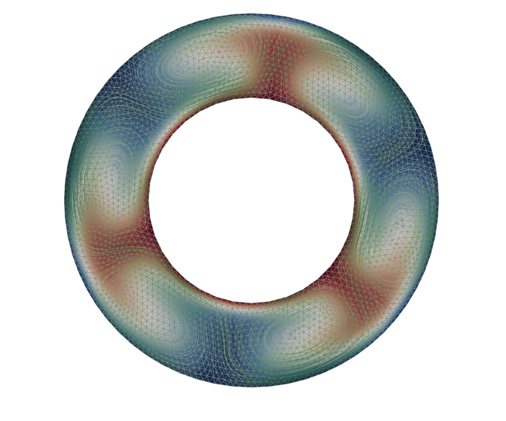
# pl.show(cpos="xy", jupyter_backend="trame")from IPython.display import IFrame
IFrame(src="html5/annulus_convection_plot.html", width=500, height=400)Interactive Image: Convection model output
Exercise - Null space
Based on our previous notebook, can you see how to calculate and (if necessary) remove rigid-body the rotation null-space from the solution ?
The use of a coarse-level singular-value decomposition for the velocity solver should help, in this case, but sometimes you can see that there is a rigid body rotation (look at the streamlines). It’s wise to check and quantify the presence of the null space.
stokes.petsc_options["fieldsplit_velocity_mg_coarse_pc_type"] = "svd"Exercise - Heat flux
Could you calculate the radial heat flux field ? Its surface average value plotted against time tells you if you have reached a steady state.
Hint:
\[ Q_\textrm{surf} = \nabla T \cdot \hat{r} + T (\mathbf{v} \cdot \hat{r} ) \]
    Q_surf = -meshball.vector.gradient(t_soln.sym).dot(unit_rvec) +\
                    t_soln.sym[0] * v_soln.sym.dot(unit_rvec)
References
Schubert, G., Turcotte, D. L., & Olson, P. (2001). Mantle Convection in the Earth and Planets (1st ed.). Cambridge University Press. https://doi.org/10.1017/CBO9780511612879