Next Steps
Underworld Documentation and Examples
In addition to the notebooks in this brief set of examples, there are a number of sources of information on using Underworld3 that you can access:
The API documentation (all the modules and functions and their full sets of arguments) is automatically generated from the source code and uses the same rich markdown content as the notebook help text.
The
underworld3GitHub repository is the most active development community for the code.
Benchmarks
The Underworld3 Benchmarks Repository is a useful place to find community benchmarks coded in underworld3 along with accuracy and convergence analysis. This is an open repository where you can make a pull request with new benchmark submissions once you get the hang of things.
The Underworld Community
The Underworld Community organisation on Github is a collection of contributed repositories from the underworld user community for all versions of the code and now includes scripts for underworld3.
Parallel Execution
Underworld3 is inherently parallel and designed for high performance computing. The symbolic layer is a relatively thin veneer that sits on top of the PETSc machinery. A script that has been developed in jupyter should be transferrable to an HPC environment with no changes (except that inherently serial operations such as visualisation and model reduction are best left to postprocessing / co-processing).
We recommend installing jupytext which allows either a seamless two-way conversion (or pairing) between the ipynb format and an annotated python script, or the ability to work entirely with annoted python scripts and not use ipynb at all. The python form does not store the output of notebook cells but there are advantages to this when scripts are under version control.
Almost all of our notebook examples are annotated python for this reason.An exception is the collection of notebooks in this quick-start guide because we want to show you the rendered output in the static web pages.
mpirun -np 1024 python3 Modelling_Script.py -uw_resolution 96The main difference between the notebook development environment and HPC is the lack of interactivity, particularly in sending parameters to the script at launch time. Typically, we expect the HPC version to be running at much higher resolution, or for many more timesteps than the development notebook. We use the PETSc command line parsing machinery to generate notebooks that also can ingest run-time parameters from a script (as above).
Parallel scaling / performance
Running geodynamic models on a single CPU/processor (i.e. serial) is time-consuming and limits us to low resolution. Underworld is build from the ground-up as a parallel computing solution which means we can easily run large models on high performance computing clusters (HPC); that is, sub-divide the problem into many smaller chunks and use multiple processors to solve each one, taking care to combine and synchronise the answers from each processor to obtain the correct solution to the original problem.
Parallel computation can reduce time we need to wait for the our results to be computed but it does happen at the expense of some overhead The overhead does depend on the nature of the computer we are using but typically we need to think about:
Code complexity: any time we manage computations across different processors, we have additional coding to reassemble the calculations correctly and we need to think about many special cases. For example, integrating a quantity of the surface of a mesh: many processes contribute, some do not, the results have to be computed independently then combined.
Additional memory is often required: to manage copies of information that lives on / near boundaries, to store the topology of the decomposed domain and to help navigate the passing of information between processes.
The time taken to synchronise results and the work required to keep track of who is doing what, when they are done, and in making sure everyone waits for everyone else. There is a time-cost in actually sending information as part of a synchronisation and a computational cost in ensuring that work is distributed efficiently.
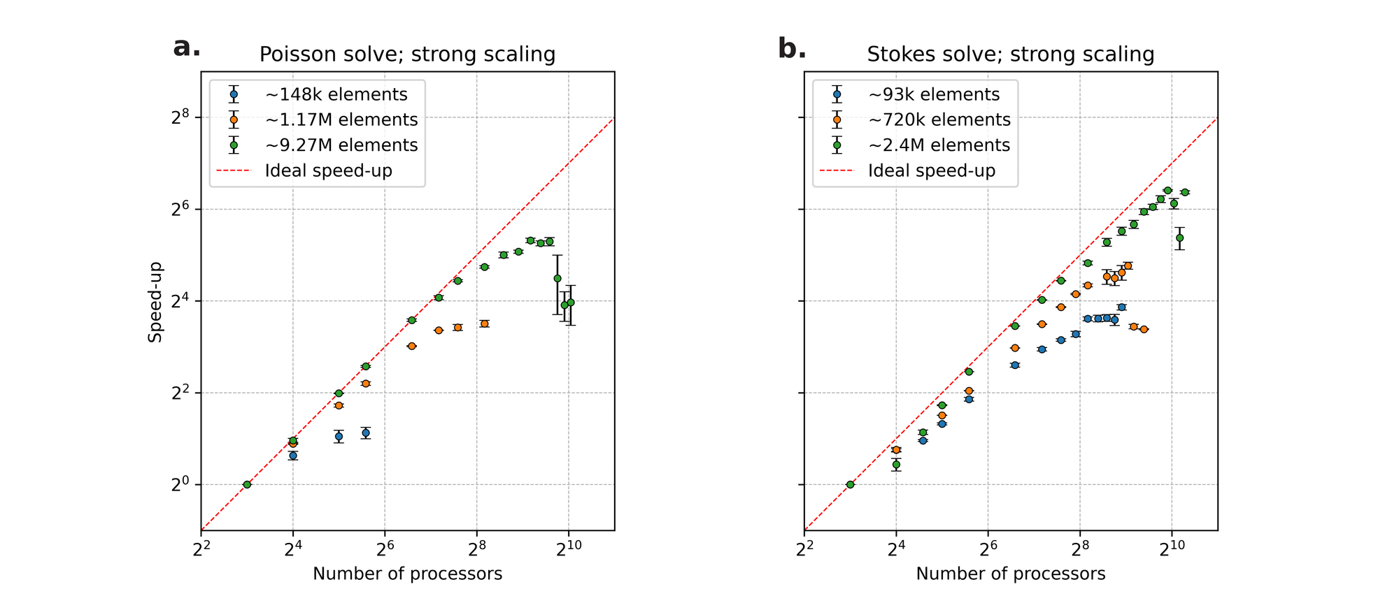
To determine the efficiency of parallel computation, we introduce the strong scaling test which measures the time taken to solve a problem in parallel compared to the same problem solved in serial. In strong scaling tests, the size of the problem is kept constant, while the number of processors is increased. The reduction in run-time due to the addition of more processors is commonly expressed in terms of the speed-up:
\[ \textrm{speed up} = \frac{t(N_{ref})}{t(N)} \]
where \(t(N_{ref})\) is the run-time for a reference number of processors, \(N_{ref}\), and \(t(N)\) is the run-time when \(N\) processors are used. In the ideal case, \(N\) additional processors should contribute all of its resources in solving the problem and reduce the compute time by a factor of \(N\) relative to the reference run time. For example, using \(2 N_{ref}\) processors will ideally halve the run-time resulting to a speed-up = 2.
Advanced capabilities
Digging a bit deeper into underworld3, there are many capabilities that require a clear understanding of the concepts that underlie the implementation. The following examples are not plug-and-play, but they do only require python coding using the underworld3 API and no detailed knowledge of petsc4py or PETSc. Get in touch with us if you want to try this sort of thing but can’t figure it out for yourself.
Deforming meshes
In Example 8, we made small variations to the mesh to conform to basal topography. We did not remesh, so we had to be careful to apply a smooth, analytic displacement to every node. For more general free-surface models, we need to calculate a smooth function using the computed boundary motions (e.g, solving a poisson equation with known boundary displacements as boundary conditions). We need to step through time and it is common to stabilize the surface motions through a surface integral term that accounts for the interface displacement during the timestep. The example below shows an underworld3 forward model with internal loads timestepped close to isostatic equilibrium.
In a more general case, we need to account to horizontal motions. This is more complicated because the horizontal velocities can be large even when vertical equilibrium is achieved. So we need to solve for the advected component of vertical motion in addition to the local component. Hooray for symbolic algebra !
Weak / penalty boundary conditions
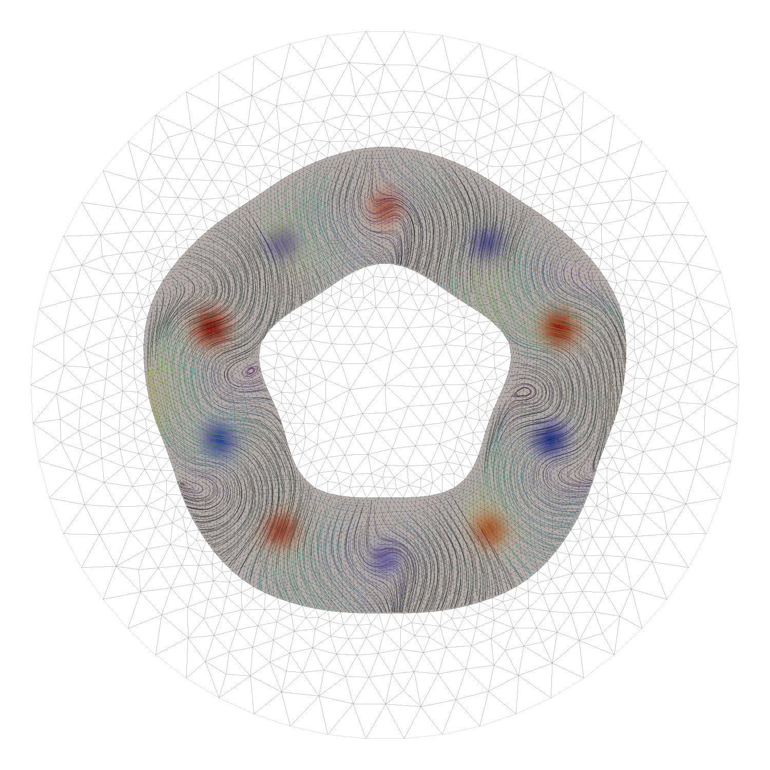
Example 8 introduced the idea of penalty-based boundary conditions where the constraint is weakly enforced by providing a large penalty for violation of the condition. This is very flexible as the penalizing conditions can be adjusted during the run, including changing which part of the boundary is subject to constraints based on the solution or a coupled problem. The channel flow model shown below has a boundary condition that depends on a externally sourced model for ponded material at the base that is derived from a simple topography filling algorithm.
Live Image: Stokes flow in a channel with multiple obstructions. Flow is driven from the inlet (a velocity boundary condition). The geometry was contructed with gmsh. This is an example for education which demonstrates the emergence of an large-scale pressure gradient as a result of the presence of the obstructions, and also the dispersion of tracers through the complicated flow geometry
The penalty approach does allow the solution to deviate from the exact value of the boundary condition, in a similar way to the iterative solvers delivering a solution to within a specified tolerance. There are some cases, for example, enforcing plate motions at the surface, where there are uncertainties in the applied boundary conditions and that these uncertainties may vary in space and time.
Mesh Adaptation
It is also possible to use the PETSc mesh adaption capabilities, to refine the resolution of a model where it is most needed and coarsen elsewhere. Dynamically-adapting meshes are possible but the interface is very low level at present, particularly in parallel.
Live Image: Static mesh adaptation to the slope of a field. The driving buoyancy term is a plume-like upwelling and the slope of this field is shown in colour (red high, blue low). Don’t forget to zoom in !
    # t is the driving "temperature". We form an isotropic refinement metric from its slope

    refinement_fn = 1.0 + sympy.sqrt(
          t.diff(x) ** 2
        + t.diff(y) ** 2
        + t.diff(z) ** 2
    )

    icoord, meshA = adaptivity.mesh_adapt_meshVar(mesh0, refinement_fn, Metric, redistribute=True)