Example 4 - `stripy` gradients on the sphere¶

SSRFPACK is a Fortran 77 software package that constructs a smooth interpolatory or approximating surface to data values associated with arbitrarily distributed points on the surface of a sphere. It employs automatically selected tension factors to preserve shape properties of the data and avoid overshoot and undershoot associated with steep gradients.

The next example is Ex5-Smoothing

Define a computational mesh¶

Use the (usual) icosahedron with face points included.

import stripy as stripy

mesh = stripy.spherical_meshes.icosahedral_mesh(refinement_levels=4, include_face_points=True)

print(mesh.npoints)

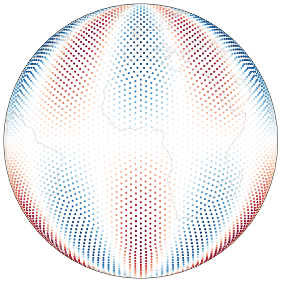
Analytic function¶

Define a relatively smooth function that we can interpolate from the coarse mesh to the fine mesh and analyse

import numpy as np

def analytic(lons, lats, k1, k2):
     return np.cos(k1*lons) * np.sin(k2*lats)

def analytic_ddlon(lons, lats, k1, k2):
     return -k1 * np.sin(k1*lons) * np.sin(k2*lats) / np.cos(lats)

def analytic_ddlat(lons, lats, k1, k2):
     return k2 * np.cos(k1*lons) * np.cos(k2*lats) 

analytic_sol = analytic(mesh.lons, mesh.lats, 5.0, 2.0)
analytic_sol_ddlon = analytic_ddlon(mesh.lons, mesh.lats, 5.0, 2.0)
analytic_sol_ddlat = analytic_ddlat(mesh.lons, mesh.lats, 5.0, 2.0)

%matplotlib inline

import cartopy
import cartopy.crs as ccrs
import matplotlib.pyplot as plt


fig = plt.figure(figsize=(10, 10), facecolor="none")
ax  = plt.subplot(111, projection=ccrs.Orthographic(central_longitude=0.0, central_latitude=0.0, globe=None))
ax.coastlines(color="lightgrey")
ax.set_global()

lons0 = np.degrees(mesh.lons)
lats0 = np.degrees(mesh.lats)

ax.scatter(lons0, lats0, 
            marker="o", s=10.0, transform=ccrs.PlateCarree(), c=analytic_sol, cmap=plt.cm.RdBu)

pass

Derivatives of solution compared to analytic values¶

The gradient_lonlat method of the sTriangulation takes a data array reprenting values on the mesh vertices and returns the lon and lat derivatives. There is an equivalent gradient_xyz method which returns the raw derivatives in Cartesian form. Although this is generally less useful, if you are computing the slope (for example) that can be computed in either coordinate system and may cross the pole, consider using the Cartesian form.

stripy_ddlon, stripy_ddlat = mesh.gradient_lonlat(analytic_sol)

## This can be an issue on jupyterhub

from xvfbwrapper import Xvfb
vdisplay = Xvfb()
try:
    vdisplay.start()
    xvfb = True

except:
    xvfb = False

---------------------------------------------------------------------------
OSError                                   Traceback (most recent call last)
<ipython-input-5-9769249b4715> in <module>
      2 
      3 from xvfbwrapper import Xvfb
----> 4 vdisplay = Xvfb()
      5 try:
      6     vdisplay.start()

~/miniconda3/envs/conda-build-docs/lib/python3.7/site-packages/xvfbwrapper.py in __init__(self, width, height, colordepth, tempdir, **kwargs)
     39         if not self.xvfb_exists():
     40             msg = 'Can not find Xvfb. Please install it and try again.'
---> 41             raise EnvironmentError(msg)
     42 
     43         self.extra_xvfb_args = ['-screen', '0', '{}x{}x{}'.format(

OSError: Can not find Xvfb. Please install it and try again.

import lavavu


lv = lavavu.Viewer(border=False, background="#FFFFFF", resolution=[1000,600], near=-10.0)

nodes = lv.points("nodes", pointsize=3.0, pointtype="shiny", colour="#448080", opacity=0.75)
nodes.vertices(mesh.points)

tris = lv.triangles("triangles",  wireframe=False, colour="#77ff88", opacity=1.0)
tris.vertices(mesh.points)
tris.indices(mesh.simplices)
tris.values(analytic_sol, label="original")
tris.values(stripy_ddlon, label="ddlon")
tris.values(stripy_ddlat, label="ddlat")
tris.values(stripy_ddlon-analytic_sol_ddlon, label="ddlonerr")
tris.values(stripy_ddlat-analytic_sol_ddlat, label="ddlaterr")


tris.colourmap("#990000 #FFFFFF #000099")
cb = tris.colourbar()

# view the pole

lv.translation(0.0, 0.0, -3.0)
lv.rotation(-20, 0.0, 0.0)

lv.control.Panel()
lv.control.Range('specular', range=(0,1), step=0.1, value=0.4)
lv.control.Checkbox(property='axis')
lv.control.ObjectList()
tris.control.List(options=["original", "ddlon", "ddlat", "ddlonerr", "ddlaterr"], property="colourby", value="original", command="redraw", label="Display:")
lv.control.show()

LavaVu Run error: Error creating OpenGL context