Litho 1.0 global sampling
Here we show how to extract information on depths of particular interfaces in the model at any point and the mechanism by which this is implemented in the wrapper.
We also demonstrate the mechanism to query a depth profile at any lon/lat location and therefore how to construct a depth profile along a great circle.
import litho1pt0 as litho
from pprint import pprint as pprint
import numpy as np

%matplotlib inline

import matplotlib.pyplot as plt
import cartopy
import cartopy.crs as ccrs
import pyproj

import stripy
pprint(" Layer keys")
pprint( litho.l1_layer_decode.items() )
pprint(" Value keys")
pprint( litho.l1_data_decode.items() )
' Layer keys'
odict_items([('ASTHENO-TOP', 0), ('LID-BOTTOM', 1), ('LID-TOP', 2), ('CRUST3-BOTTOM', 3), ('CRUST3-TOP', 4), ('CRUST2-BOTTOM', 5), ('CRUST2-TOP', 6), ('CRUST1-BOTTOM', 7), ('CRUST1-TOP', 8), ('SEDS3-BOTTOM', 9), ('SEDS3-TOP', 10), ('SEDS2-BOTTOM', 11), ('SEDS2-TOP', 12), ('SEDS1-BOTTOM', 13), ('SEDS1-TOP', 14), ('WATER-BOTTOM', 15), ('WATER-TOP', 16), ('ICE-BOTTOM', 17), ('ICE-TOP', 18)])
' Value keys'
odict_items([('DEPTH', 0), ('DENSITY', 1), ('VP', 2), ('VS', 3), ('QKAPPA', 4), ('QMU', 5), ('VP2', 6), ('VS2', 7), ('ETA', 8)])
lats = np.array([0,0,0,0])
lons = np.array([10,10,10,10])
depths = np.array([1, 20, 100, 1000 ])


C, Vp = litho.property_at_lat_lon_depth_points(lats, lons, depths, quantity_ID='VP')

print (C)
print (Vp)
[8 6 2 0]
[6454 6663 8127 7965]
## Checking the integrity

nlayers = len(litho.l1_layer_decode)
layer_depths     = np.empty((nlayers, lats.shape[0]))
layer_properties = np.empty((nlayers, lats.shape[0]))

for i in range(0, nlayers, 1 ):
    layer_depths[i], err =  litho._interpolator.interpolate(lons * np.pi / 180.0, lats * np.pi / 180.0,
                                                  litho._litho_data[i,litho.l1_data_decode["DEPTH"]], order=1)

    layer_properties[i], err = litho._interpolator.interpolate( lons * np.pi / 180.0, lats * np.pi / 180.0,
                                          litho._litho_data[i,litho.l1_data_decode["DENSITY"]], order=1)


print (layer_depths)
print (layer_properties)
[[ 2.23957740e+05  2.23957740e+05  2.23957740e+05  2.23957740e+05]
 [ 2.23957740e+05  2.23957740e+05  2.23957740e+05  2.23957740e+05]
 [ 3.70932548e+04  3.70932548e+04  3.70932548e+04  3.70932548e+04]
 [ 3.70932548e+04  3.70932548e+04  3.70932548e+04  3.70932548e+04]
 [ 2.40532913e+04  2.40532913e+04  2.40532913e+04  2.40532913e+04]
 [ 2.40532913e+04  2.40532913e+04  2.40532913e+04  2.40532913e+04]
 [ 1.10133277e+04  1.10133277e+04  1.10133277e+04  1.10133277e+04]
 [ 1.10133277e+04  1.10133277e+04  1.10133277e+04  1.10133277e+04]
 [ 8.71133817e+02  8.71133817e+02  8.71133817e+02  8.71133817e+02]
 [ 8.71133817e+02  8.71133817e+02  8.71133817e+02  8.71133817e+02]
 [ 8.71133817e+02  8.71133817e+02  8.71133817e+02  8.71133817e+02]
 [ 8.71133817e+02  8.71133817e+02  8.71133817e+02  8.71133817e+02]
 [ 1.82232094e+02  1.82232094e+02  1.82232094e+02  1.82232094e+02]
 [ 1.82232094e+02  1.82232094e+02  1.82232094e+02  1.82232094e+02]
 [-1.28888395e+02 -1.28888395e+02 -1.28888395e+02 -1.28888395e+02]
 [-1.28888395e+02 -1.28888395e+02 -1.28888395e+02 -1.28888395e+02]
 [-1.28888395e+02 -1.28888395e+02 -1.28888395e+02 -1.28888395e+02]
 [-1.28888395e+02 -1.28888395e+02 -1.28888395e+02 -1.28888395e+02]
 [-1.28888395e+02 -1.28888395e+02 -1.28888395e+02 -1.28888395e+02]]
[[  3300.           3300.           3300.           3300.        ]
 [  3300.           3300.           3300.           3300.        ]
 [  3300.           3300.           3300.           3300.        ]
 [  3029.63347697   3029.63347697   3029.63347697   3029.63347697]
 [  3029.63347697   3029.63347697   3029.63347697   3029.63347697]
 [  2925.52236093   2925.52236093   2925.52236093   2925.52236093]
 [  2925.52236093   2925.52236093   2925.52236093   2925.52236093]
 [  2873.4668029    2873.4668029    2873.4668029    2873.4668029 ]
 [  2873.4668029    2873.4668029    2873.4668029    2873.4668029 ]
 [-99999.         -99999.         -99999.         -99999.        ]
 [-99999.         -99999.         -99999.         -99999.        ]
 [  2359.99955575   2359.99955575   2359.99955575   2359.99955575]
 [  2359.99955575   2359.99955575   2359.99955575   2359.99955575]
 [  2102.2218767    2102.2218767    2102.2218767    2102.2218767 ]
 [  2102.2218767    2102.2218767    2102.2218767    2102.2218767 ]
 [-99999.         -99999.         -99999.         -99999.        ]
 [-99999.         -99999.         -99999.         -99999.        ]
 [-99999.         -99999.         -99999.         -99999.        ]
 [-99999.         -99999.         -99999.         -99999.        ]]
## make a global raster of some quantity

lonv, latv = np.meshgrid(np.linspace(-180,180,360), np.linspace(-90,90,180), sparse=False, indexing='xy')

l1 = litho.layer_depth(latv, lonv, "LID-BOTTOM")
l2 = litho.layer_depth(latv, lonv, "LID-TOP")

lthickness = (l1 - l2)*0.001

l1 = litho.layer_depth(latv, lonv, "CRUST3-BOTTOM")
l2 = litho.layer_depth(latv, lonv, "CRUST1-TOP")

cthickness = (l1 - l2)*0.001

# density at 1km depth
depths = np.ones_like(lonv, dtype=np.float)*5.0

ids, density_at_1km = litho.property_at_lat_lon_depth_points(latv, lonv, depths, quantity_ID="DENSITY")
%matplotlib inline

import cartopy
import gdal
import cartopy.crs as ccrs
import matplotlib.pyplot as plt

projection1 = ccrs.Orthographic(central_longitude=140.0, central_latitude=0.0, globe=None)
projection2 = ccrs.Mollweide(central_longitude=0)
base_projection = ccrs.PlateCarree()

global_extent     = [-180.0, 180.0, -90.0, 90.0]


fig = plt.figure(figsize=(12, 12), facecolor="none")
ax  = plt.subplot(111, projection=projection2)
ax.coastlines()
ax.set_global()

m = ax.imshow(density_at_1km.reshape(-1,360), origin='lower', transform=base_projection,
              extent=global_extent, zorder=0, cmap="Blues")

plt.colorbar(mappable=m, orientation="horizontal", shrink=0.5)
---------------------------------------------------------------------------
ModuleNotFoundError                       Traceback (most recent call last)
<ipython-input-6-f26ad715993a> in <module>
      2
      3 import cartopy
----> 4 import gdal
      5 import cartopy.crs as ccrs
      6 import matplotlib.pyplot as plt

ModuleNotFoundError: No module named 'gdal'
def great_circle_profile(startlonlat, endlonlat, depths, resolution, QID):
    """
    model: self
    ll0: (lon0, lat0)
    ll1: (lon1, lat1)
    depths (km)
    resolution: separation (km) of locations to sample along the profile
    """

    import stripy

    lons, lats = great_circle_Npoints(np.radians(startlonlat), np.radians(endlonlat), 1000)

    ## Would be useful to have distance measure here to map resolutions ...

    data = np.empty( (lons.shape[0], depths.shape[0]))

    for s, ll in enumerate(lons):
        c, profile = litho.property_on_depth_profile(np.degrees(lats[s]), np.degrees(lons[s]), depths, QID)
        data[s,:] = profile[:]


    return np.degrees(lons), np.degrees(lats), data


def great_circle_Npoints(lonlat1, lonlat2, N):
    """
    N points along the line joining lonlat1 and lonlat2
    """

    ratio = np.linspace(0.0,1.0, N).reshape(-1,1)

    lonlat1r = np.radians(lonlat1)
    lonlat2r = np.radians(lonlat2)


    xyz1 = np.array(stripy.spherical.lonlat2xyz(lonlat1r[0], lonlat1r[1])).T
    xyz2 = np.array(stripy.spherical.lonlat2xyz(lonlat2r[0], lonlat2r[1])).T

    mids = ratio * xyz2 + (1.0-ratio) * xyz1
    norm = (mids**2).sum(axis=1)
    xyzN = mids / norm.reshape(-1,1)

    lonlatN = stripy.spherical.xyz2lonlat( xyzN[:,0], xyzN[:,1], xyzN[:,2])

    return np.degrees(lonlatN)
depths = np.linspace(-10.0, 250, 100)
startlonlat=np.array([80.0,5.0])
endlonlat  =np.array([80.0,45.0])

midlonlat = 0.5 * ( startlonlat + endlonlat)

lons, lats, d = great_circle_profile(startlonlat, endlonlat, depths, 2.5, "DENSITY")
lonlat1r = np.radians(startlonlat)
lonlat2r = np.radians(endlonlat)
xyz1 = np.array(stripy.spherical.lonlat2xyz(lonlat1r[0], lonlat1r[1])).T
xyz2 = np.array(stripy.spherical.lonlat2xyz(lonlat2r[0], lonlat2r[1])).T

N=100
ratio = np.linspace(0.0,1.0, N).reshape(-1,1)
mids = ratio * xyz2 + (1.0-ratio) * xyz1
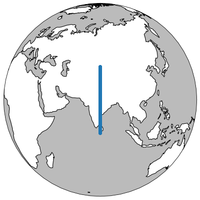
fig = plt.figure(figsize=(7, 7), facecolor="none")

ax  = plt.subplot(111, projection=ccrs.Orthographic(central_latitude=midlonlat[1], central_longitude=midlonlat[0]))
ax.set_global()

ax.add_feature(cartopy.feature.OCEAN, alpha=1.0, facecolor="#BBBBBB", zorder=0)
ax.scatter(lons, lats, transform=ccrs.PlateCarree(), zorder=100)

ax.coastlines()
<cartopy.mpl.feature_artist.FeatureArtist at 0x7fa3daf0ac50>
/Users/runner/miniconda3/envs/conda-build-docs/lib/python3.7/site-packages/cartopy/io/__init__.py:260: DownloadWarning: Downloading: https://naciscdn.org/naturalearth/110m/physical/ne_110m_coastline.zip
  warnings.warn('Downloading: {}'.format(url), DownloadWarning)
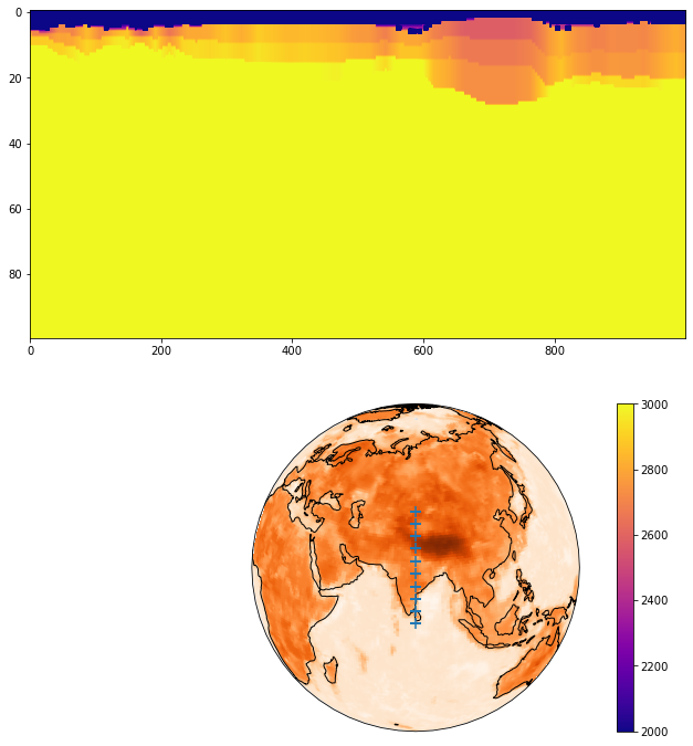
# Compute some properties about the profile line itself

drange = depths[-1] - depths[0]

#
# Cross section
#

fig = plt.figure(figsize=(12, 12), facecolor="none")
ax  = plt.subplot(211)
ax2 = plt.subplot(212, projection=ccrs.Orthographic(central_latitude=midlonlat[1],
                                                    central_longitude=midlonlat[0]))

image = d[:,:]
m1 = ax.imshow(image.T, origin="upper", cmap="plasma", aspect=5.0, vmin=2000, vmax=3000)

plt.colorbar(mappable=m1, )


#
# Map / cross section
#

ax2.set_global()
global_extent     = [-180.0, 180.0, -90.0, 90.0]
m = ax2.imshow(cthickness, origin='lower', transform=ccrs.PlateCarree(),
              extent=global_extent, zorder=0, cmap="Oranges")


ax2.add_feature(cartopy.feature.OCEAN, alpha=0.25, facecolor="#BBBBBB")
ax2.coastlines()

lonr, latr = great_circle_Npoints(np.radians(startlonlat), np.radians(endlonlat), 10)
ptslo  = np.degrees(lonr)
ptsla  = np.degrees(latr)

ax2.scatter (ptslo, ptsla, marker="+", s=100, transform=ccrs.PlateCarree(), zorder=101)
<matplotlib.collections.PathCollection at 0x7fa3d8f4e350>