Example 2 - stripy predefined meshes
One common use of stripy is in meshing the sphere and, to this end, we provide pre-defined meshes for icosahedral and octahedral triangulations, each of which can have mid-face centroid points included. A triangulation of the six cube-vertices is also provided as well as a ‘buckyball’ (or ‘soccer ball’) mesh. A random mesh is included as a counterpoint to the regular meshes. Each of these meshes is also an sTriangulation.
The mesh classes in stripy are:
stripy.spherical_meshes.octahedral_mesh(include_face_points=False)
stripy.spherical_meshes.icosahedral_mesh(include_face_points=False)
stripy.spherical_meshes.triangulated_cube_mesh()
stripy.spherical_meshes.triangulated_soccerball_mesh()
stripy.spherical_meshes.uniform_ring_mesh(resolution=5)
stripy.spherical_meshes.random_mesh(number_of_points=5000)
Any of the above meshes can be uniformly refined by specifying the refinement_levels parameter.
Sample meshes
We create a number of meshes from the basic types available in stripy with approximately similar numbers of vertices.
import stripy as stripy

str_fmt = "{:35} {:3}\t{:6}"


## A bunch of meshes with roughly similar overall numbers of points / triangles

octo0  = stripy.spherical_meshes.octahedral_mesh(include_face_points=False, refinement_levels=0)
octo2  = stripy.spherical_meshes.octahedral_mesh(include_face_points=False, refinement_levels=2)
octoR  = stripy.spherical_meshes.octahedral_mesh(include_face_points=False, refinement_levels=5)

print(str_fmt.format("Octahedral mesh", octo0.npoints, octoR.npoints))


octoF0  = stripy.spherical_meshes.octahedral_mesh(include_face_points=True, refinement_levels=0)
octoF2  = stripy.spherical_meshes.octahedral_mesh(include_face_points=True, refinement_levels=2)
octoFR  = stripy.spherical_meshes.octahedral_mesh(include_face_points=True, refinement_levels=4)

print(str_fmt.format("Octahedral mesh with faces", octoF0.npoints, octoFR.npoints))


cube0 = stripy.spherical_meshes.triangulated_cube_mesh(refinement_levels=0)
cube2 = stripy.spherical_meshes.triangulated_cube_mesh(refinement_levels=2)
cubeR = stripy.spherical_meshes.triangulated_cube_mesh(refinement_levels=5)

print(str_fmt.format("Cube mesh", cube0.npoints, cubeR.npoints))


ico0 = stripy.spherical_meshes.icosahedral_mesh(refinement_levels=0)
ico2 = stripy.spherical_meshes.icosahedral_mesh(refinement_levels=2)
icoR = stripy.spherical_meshes.icosahedral_mesh(refinement_levels=4)

print(str_fmt.format("Icosahedral mesh", ico0.npoints, icoR.npoints))


icoF0 = stripy.spherical_meshes.icosahedral_mesh(refinement_levels=0, include_face_points=True)
icoF2 = stripy.spherical_meshes.icosahedral_mesh(refinement_levels=2, include_face_points=True)
icoFR = stripy.spherical_meshes.icosahedral_mesh(refinement_levels=4, include_face_points=True)

print(str_fmt.format("Icosahedral mesh with faces", icoF0.npoints, icoFR.npoints))


socc0 = stripy.spherical_meshes.triangulated_soccerball_mesh(refinement_levels=0)
socc2 = stripy.spherical_meshes.triangulated_soccerball_mesh(refinement_levels=1)
soccR = stripy.spherical_meshes.triangulated_soccerball_mesh(refinement_levels=3)

print(str_fmt.format("BuckyBall mesh", socc0.npoints, soccR.npoints))


## Need a reproducible hierarchy ...
ring0 = stripy.spherical_meshes.uniform_ring_mesh(resolution=5, refinement_levels=0)

lon, lat = ring0.uniformly_refine_triangulation()
ring1 = stripy.sTriangulation(lon, lat)

lon, lat = ring1.uniformly_refine_triangulation()
ring2 = stripy.sTriangulation(lon, lat)

lon, lat = ring2.uniformly_refine_triangulation()
ring3 = stripy.sTriangulation(lon, lat)

lon, lat = ring3.uniformly_refine_triangulation()
ringR = stripy.sTriangulation(lon, lat)


# ring2 = stripy.uniform_ring_mesh(resolution=6, refinement_levels=2)
# ringR = stripy.uniform_ring_mesh(resolution=6, refinement_levels=4)

print(str_fmt.format("Ring mesh (9)", ring0.npoints, ringR.npoints))

randR = stripy.spherical_meshes.random_mesh(number_of_points=5000)
rand0 = stripy.sTriangulation(lons=randR.lons[::50],lats=randR.lats[::50])
rand2 = stripy.sTriangulation(lons=randR.lons[::25],lats=randR.lats[::25])

print(str_fmt.format("Random mesh (6)", rand0.npoints, randR.npoints))
Octahedral mesh                       6	  4098
Octahedral mesh with faces           14	  3074
Cube mesh                             8	  6146
Icosahedral mesh                     12	  2562
Icosahedral mesh with faces          32	  7682
BuckyBall mesh                       92	  5762
Ring mesh (9)                        30	  7170
Random mesh (6)                     100	  5000
print("Octo: {}".format(octo0.__doc__))
print("Cube: {}".format(cube0.__doc__))
print("Ico: {}".format(ico0.__doc__))
print("Socc: {}".format(socc0.__doc__))
print("Ring: {}".format(ring0.__doc__))
print("Random: {}".format(randR.__doc__))
Octo:
    An octahedral triangulated mesh based on the sTriangulation class

Cube:
    An cube-based triangulated mesh based on the sTriangulation class

Ico:
    An icosahedral triangulated mesh based on the sTriangulation class.

Socc:
    This mesh is inspired by the C60 molecule and the soccerball - a truncated
    icosahedron with mid points added to all pentagon and hexagon faces to create
    a uniform triangulation.

Ring:
    A mesh of made of rings to create a roughly gridded, even spacing on
    the sphere. There is a small random component to prevent points lying along the
    prime meridian so this mesh should be used with caution in parallel

Random:
    A mesh of random points. Take care if you use this is parallel
    as the location of points will not be the same on all processors
Analysis of the characteristics of the triangulations
We plot a histogram of the (spherical) areas of the triangles in each of the triangulations normalised by the average area. This is one measure of the uniformity of each mesh.
%matplotlib inline
import matplotlib.pyplot as plt
import numpy as np

def area_histo(mesh):

    freq, area_bin = np.histogram(mesh.areas(), bins=20)
    area = 0.5 * (area_bin[1:] + area_bin[:-1])
    (area * freq)
    norm_area = area / mesh.areas().mean()

    return norm_area, 0.25 * freq*area / np.pi**2

def add_plot(axis, mesh, xlim, ylim):
    u, v = area_histo(mesh)
    axis.bar(u, v, width=0.025)
    axis.set_xlim(xlim)
    axis.set_ylim(ylim)
    axis.plot([1.0,1.0], [0.0,1.5], linewidth=1.0, linestyle="-.", color="Black")

    return


fig, ax = plt.subplots(4,2, sharey=True, figsize=(8,16))

xlim=(0.75,1.5)
ylim=(0.0,0.125)

# octahedron

add_plot(ax[0,0], octoR, xlim, ylim)

# octahedron + faces

add_plot(ax[0,1], octoFR, xlim, ylim)


# icosahedron

add_plot(ax[1,0], icoR, xlim, ylim)

# icosahedron + faces

add_plot(ax[1,1], icoFR, xlim, ylim)


# cube

add_plot(ax[2,0], cubeR, xlim, ylim)

# C60

add_plot(ax[2,1], soccR, xlim, ylim)


# ring

add_plot(ax[3,0], ringR, xlim, ylim)

# random (this one is very different from the others ... )

axis=ax[3,1]
u, v = area_histo(randR)
axis.bar(u, v, width=0.5)
axis.set_xlim(0.0,11.0)
axis.set_ylim(0,0.125)
axis.plot([1.0,1.0], [0.0,1.5], linewidth=1.0, linestyle="-.", color="Black")


fig.savefig("AreaDistributionsByMesh.png", dpi=250, transparent=True)


#ax.bar(norm_area, area*freq, width=0.01)
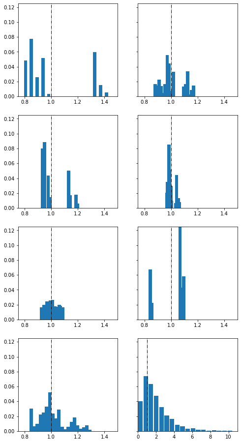
The icosahedron with faces looks like this
It is helpful to be able to view a mesh in 3D to verify that it is an appropriate choice. Here, for example, is the icosahedron with additional points in the centroid of the faces.
This produces triangles with a narrow area distribution. In three dimensions it is easy to see the origin of the size variations.
## The icosahedron with faces in 3D view

import lavavu

from xvfbwrapper import Xvfb
with Xvfb() as xvfb:

    ## or smesh = icoF0
    smesh = icoFR

    lv = lavavu.Viewer(border=False, background="#FFFFFF", resolution=[1000,600], near=-10.0)

    tris = lv.triangles("triangulation",  wireframe=True, colour="#444444", opacity=0.8)
    tris.vertices(smesh.points)
    tris.indices(smesh.simplices)

    tris2 = lv.triangles("triangles",  wireframe=False, colour="#77ff88", opacity=0.8)
    tris2.vertices(smesh.points)
    tris2.indices(smesh.simplices)

    nodes = lv.points("nodes", pointsize=2.0, pointtype="shiny", colour="#448080", opacity=0.75)
    nodes.vertices(smesh.points)


    lv.control.Panel()
    lv.control.Range('specular', range=(0,1), step=0.1, value=0.4)
    lv.control.Checkbox(property='axis')
    lv.control.ObjectList()
    lv.control.show()
---------------------------------------------------------------------------
OSError                                   Traceback (most recent call last)
<ipython-input-4-fc189566737e> in <module>
      4
      5 from xvfbwrapper import Xvfb
----> 6 with Xvfb() as xvfb:
      7
      8     ## or smesh = icoF0

~/miniconda3/envs/conda-build-docs/lib/python3.7/site-packages/xvfbwrapper.py in __init__(self, width, height, colordepth, tempdir, **kwargs)
     39         if not self.xvfb_exists():
     40             msg = 'Can not find Xvfb. Please install it and try again.'
---> 41             raise EnvironmentError(msg)
     42
     43         self.extra_xvfb_args = ['-screen', '0', '{}x{}x{}'.format(

OSError: Can not find Xvfb. Please install it and try again.
%matplotlib inline

import cartopy
import cartopy.crs as ccrs
import matplotlib.pyplot as plt

global_extent     = [-180.0, 180.0, -90.0, 90.0]

projection1 = ccrs.Orthographic(central_longitude=0.0, central_latitude=0.0, globe=None)
projection2 = ccrs.Mollweide(central_longitude=-120)
projection3 = ccrs.PlateCarree()
base_projection = ccrs.PlateCarree()
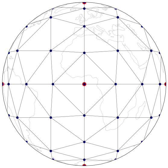
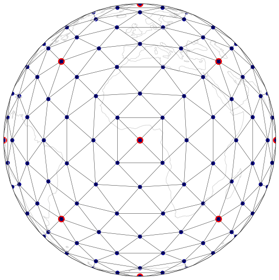
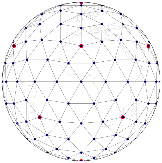
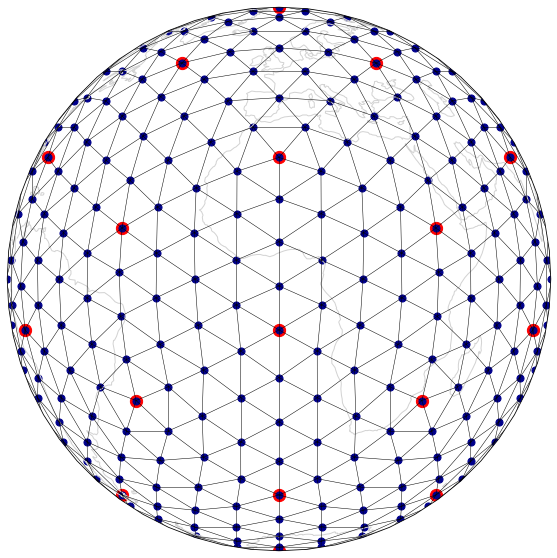
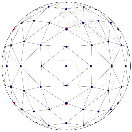
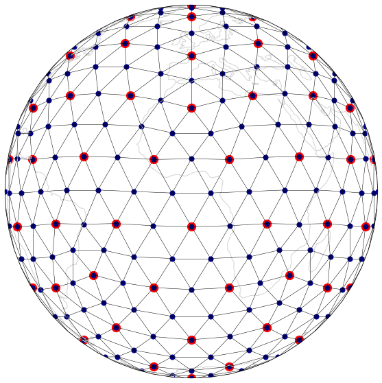
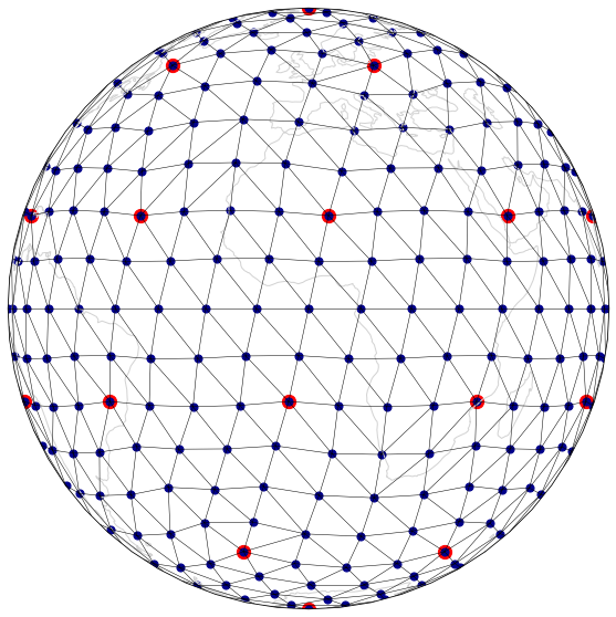
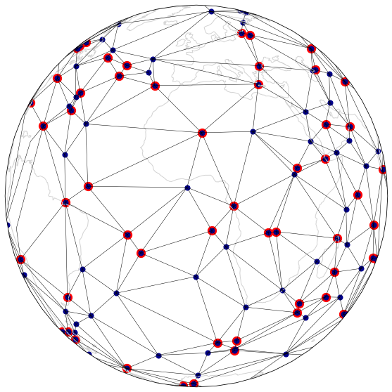
Plot and compare the predefined meshes
def mesh_fig(mesh, meshR, name):

    fig = plt.figure(figsize=(10, 10), facecolor="none")
    ax  = plt.subplot(111, projection=ccrs.Orthographic(central_longitude=0.0, central_latitude=0.0, globe=None))
    ax.coastlines(color="lightgrey")
    ax.set_global()

    generator = mesh
    refined   = meshR

    lons0 = np.degrees(generator.lons)
    lats0 = np.degrees(generator.lats)

    lonsR = np.degrees(refined.lons)
    latsR = np.degrees(refined.lats)

    lst = refined.lst
    lptr = refined.lptr


    ax.scatter(lons0, lats0, color="Red",
                marker="o", s=150.0, transform=ccrs.PlateCarree())

    ax.scatter(lonsR, latsR, color="DarkBlue",
                marker="o", s=50.0, transform=ccrs.PlateCarree())


    segs = refined.identify_segments()

    for s1, s2 in segs:
        ax.plot( [lonsR[s1], lonsR[s2]],
                 [latsR[s1], latsR[s2]],
                 linewidth=0.5, color="black", transform=ccrs.Geodetic())

    fig.savefig(name, dpi=250, transparent=True)

    return

mesh_fig(octo0,  octo2, "Octagon" )
mesh_fig(octoF0, octoF2, "OctagonF" )

mesh_fig(ico0, ico2, "Icosahedron" )
mesh_fig(icoF0, icoF2, "IcosahedronF" )

mesh_fig(cube0, cube2, "Cube")
mesh_fig(socc0, socc2, "SoccerBall")

mesh_fig(ring0, ring2, "Ring")
mesh_fig(rand0, rand2, "Random")
The next example is Ex3-Interpolation