1. Creating meshes¶

Quagmire can model surface processess on a structured rectangular grid or unstructured triangulated points. These use-cases are bundled into two objects:

PixMesh: meshing on a rectangular grid
TriMesh: meshing on unstructured triangular points
sTriMesh: meshing on unstructured triangular points on the sphere

All meshes are generated and handed to Quagmire using a DM object where the selection of PixMesh, TriMesh, or sTriMesh is identified automatically by QuagMesh. The following data structures are built:

Delaunay triangulation
node neighbour array
pointwise area and weights
boundary information
Rbf smoothing kernel

In this notebook we setup different DM objects using meshes found in the quagmire.tools.meshtools path and hand them to QuagMesh.

from quagmire.tools import meshtools
from quagmire import QuagMesh
import numpy as np

Structured grids¶

minX, maxX = -5.0, 5.0
minY, maxY = -5.0, 5.0

resX = 75
resY = 75

DM = meshtools.create_DMDA(minX, maxX, minY, maxY, resX, resY)

print(type(DM))

<class 'petsc4py.PETSc.DMDA'>

This is a native PETSc data management object for structured grids (DMDA). This object has a number of useful methods and attached data which can be listed with

help(DM)

We hand this to QuagMesh to generate the necessary data structures for gradient operations, smoothing, neighbour allocation, etc.

mesh = QuagMesh(DM)

Underlying Mesh type: PixMesh
- cKDTree 0.0034633329998996487s
- Find boundaries 0.002306667000084417s
- Construct neighbour cloud arrays 0.029511375000083717s, (0.0155398750000586s + 0.013944875000106549s)
- Construct rbf weights 0.007861209000111558s

We attach data to a mesh solely through mesh variables (see Example notebook for details)

    mesh_variable = mesh.add_variable(name="data1")
    mesh_variable.data = np.sin(mesh.coords[:,0] * np.pi)
    mesh_variable.sync()

The sync operation ensures data is coherent across processors - it is harmless and relatively inexpensive so is safe to use even in cases like this where there is no way for information to be out of sync between domains.

mesh_variable = mesh.add_variable(name="data1")
mesh_variable.data = np.sin(mesh.coords[:,0] * np.pi)
mesh_variable.sync()

mesh_variable2 = mesh.add_variable(name="data2")
mesh_variable2.data = np.sin(mesh.coords[:,0] * 0.2 * np.pi) * np.cos(mesh.coords[:,1] * 0.2 * np.pi) 
mesh_variable2.sync()

XY = mesh.coords
XYZ = np.vstack((XY[:,0],XY[:,1], mesh_variable2.data)).T

Visualisation¶

Visualisation of meshes is explained in more detail in Ex1.1-Visualising-Meshes so we will just look at the results of the visualisation for the moment.

import numpy as np
import k3d

plot = k3d.plot(camera_auto_fit=True, grid_visible=False)

plot += k3d.points(XYZ, point_size=0.05)

plot += k3d.surface(mesh_variable2.data.reshape((mesh.nx,mesh.ny)), 
                   xmin=mesh.minX, xmax=mesh.maxX, ymin=mesh.minY, ymax=mesh.maxY,
                   color=0x995500
                   )
plot.display()

/Users/lmoresi/mambaforge/envs/underworld/lib/python3.9/site-packages/traittypes/traittypes.py:97: UserWarning: Given trait value dtype "float64" does not match required type "float32". A coerced copy has been created.
  warnings.warn(

# import lavavu

# lv = lavavu.Viewer(border=False, background="#FFFFFF", resolution=[500,500], near=-10.0)

# lvmesh = lv.quads(dims=(mesh.nx, mesh.ny), wireframe=True)
# lvmesh.vertices(mesh.coords)
# lvmesh.values( mesh_variable.data, "sinx")
# lvmesh.colourmap("#FF0000, #555555 #0000FF", range=[-1.0,1.0])

# # The mesh can be given a height mapping like this

# vertices = np.zeros((mesh.coords.shape[0],3))
# vertices[:,0:2] = mesh.coords
# vertices[:,2]   = mesh_variable2.data * 0.5

# lvmesh2 = lv.quads(dims=(mesh.nx, mesh.ny), wireframe=False)
# lvmesh2.vertices(vertices)
# lvmesh2.values(mesh_variable2.data,"sinxcosy")
# lvmesh2.colourmap("#FF0000, #FFFFFF:0.5 #0000FF", range=[-1.0,1.0])


# lv.control.Panel()
# lv.control.ObjectList()
# lv.control.show()

Unstructured meshes¶

This is handled by PETSc’s DMPlex object, which requires the connectivity of a set of points. The connectivity between points can be triangulated using the built-in mesh creation tools:

x, y, simplices = square_mesh(minX, maxX, minY, maxY, spacingX, spacingY)
x, y, simplices = elliptical_mesh(minX, maxX, minY, maxY, spacingX, spacingY)

and handed to DMPlex using:

DM = meshtools.create_DMPlex(x, y, simplices, boundary_vertices=None, refinement_levels=0)

Alternatively, an arbitrary set of points (without duplicates) can be triangulated and processed as a DMPlex object using:

meshtools.create_DMPlex_from_points(x, y, bmask=None, refinement_levels=0)

If no boundary information is provided, the boundary is assumed to be the convex hull of points.

Parallel notes¶

The triangulation from the root processor is distributed to other processors using the DM object, including boundary points and boundary edges. The mesh can be refined efficiently in parallel using the refine_dm method. The order of this operation is important:

Triangulate points
Mark boundary edges
Distribute DMPlex to other processors
Refine the mesh

Elliptical mesh¶

spacingX = 0.1
spacingY = 0.1

x, y, simplices = meshtools.elliptical_mesh(minX, maxX, minY, maxY, spacingX, spacingY)
DM = meshtools.create_DMPlex(x, y, simplices)

mesh = QuagMesh(DM)

mesh_equant = mesh.neighbour_cloud_distances.mean(axis=1) / ( np.sqrt(mesh.area))

Underlying Mesh type: TriMesh
- Delaunay triangulation 0.004698625000173706s
- Calculate node weights and area 0.0006435829998281406s
- Find boundaries 0.0009458749998429994s
- cKDTree 0.0008878749999894353s
- Construct neighbour cloud arrays 0.010321582999949896s, (0.007003082999972321s + 0.0032964580000225396s)
- Construct rbf weights 0.0013669160000517877s

import k3d
plot = k3d.plot(camera_auto_fit=True,   grid_visible=False)

mesh0 = mesh
indices = mesh0.tri.simplices.astype(np.uint32)
points  = np.column_stack((mesh0.coords, mesh0.coords[:,0]*0.0)).astype(np.float32)
plt_mesh = k3d.mesh(points, indices, wireframe=True, color=0xFF8000)
plot += plt_mesh
plot.display()

Mesh improvement¶

Applies Lloyd’s algorithm of iterated voronoi construction to improve the mesh point locations. This distributes the points to a more uniform spacing with more equant triangles. It can be very slow for anything but a small mesh. Refining the mesh a few times will produce a large, well-spaced mesh.

bmask = mesh.bmask.copy()

x1, y1 = meshtools.lloyd_mesh_improvement(x, y, bmask, iterations=3)
DM = meshtools.create_DMPlex_from_points(x1, y1, bmask)

mesh1 = QuagMesh(DM)

Underlying Mesh type: TriMesh
- Delaunay triangulation 0.003389666999964902s
- Calculate node weights and area 0.00048416699996778334s
- Find boundaries 0.00044929199998478s
- cKDTree 0.00035741600004257634s
- Construct neighbour cloud arrays 0.010160874999883163s, (0.006841458000053535s + 0.0032979590000650205s)
- Construct rbf weights 0.0010214999999789143s

mesh1_equant = mesh1.neighbour_cloud_distances.mean(axis=1) / ( np.sqrt(mesh1.area))

import k3d
plot = k3d.plot(camera_auto_fit=True,   grid_visible=False)

mesh0 = mesh1
indices = mesh0.tri.simplices.astype(np.uint32)
points  = np.column_stack((mesh0.coords, mesh0.coords[:,0]*0.0)).astype(np.float32)
plt_mesh = k3d.mesh(points, indices, wireframe=True, color=0xFF8000)
                                       
plot += plt_mesh

mesh0 = mesh
points  = np.column_stack((mesh0.coords, mesh0.coords[:,0]*0.0)).astype(np.float32)
plot += k3d.points(points, point_size=0.05)

plot.display()

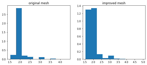
# Comparison of point-wise area for original and improved mesh

import matplotlib.pyplot as plt
%matplotlib inline

fig, (ax1, ax2) = plt.subplots(1,2, figsize=(10,4))

ax1.hist(mesh_equant, density=True)
ax2.hist(mesh1_equant, density=True)

ax1.set_title('original mesh')
ax2.set_title('improved mesh')

plt.show()

Spherical meshes¶

This unstructed mesh uses PETSc’s DMPlex object, and uses stripy to triangulate on the unit sphere. Multiple meshes may be created, including:

DM = meshtools.create_spherical_DMPlex(lons, lats, simplices, boundary_vertices=None)
DM = meshtools.create_DMPlex_from_spherical_points(lons, lats, simplices, bmask=None, refinement_levels=0)

If no boundary information is provided, the boundary is calculated from any line segments that do not share a triangle with another.a

import stripy

lons, lats, bmask = meshtools.generate_elliptical_points(-40, 40, -80, 80, 0.1, 0.1, 1500, 200)

icomesh = stripy.spherical_meshes.icosahedral_mesh(refinement_levels=5, include_face_points=True)

lons = np.degrees(icomesh.lons)
lats = np.degrees(icomesh.lats)
bmask = None

DM = meshtools.create_DMPlex_from_spherical_points(lons, lats, bmask, refinement_levels=0)
mesh0 = QuagMesh(DM)

Origin =  0.0 0.0 Radius =  40.0 Aspect =  2.0
Underlying Mesh type: sTriMesh
- Delaunay triangulation 0.049711750000142274s
- Calculate node weights and area 0.008660291000069265s
- Find boundaries 0.003692999999884705s
- cKDTree 0.004933917000016663s
- Construct neighbour cloud arrays 0.18275120899988906s, (0.14103324999996403s + 0.04168125000001055s)
- Construct rbf weights 0.014639875000057145s

b = open("GreyEarth.tif", "rb").read()

131327272

U = 0.5 + mesh0.tri.lons_map_to_wrapped(mesh0.tri.lons) / (2.0*np.pi) 
V = 0.5 - mesh0.tri.lats / np.pi

import k3d
plot = k3d.plot(camera_auto_fit=False)

indices = mesh0.tri.simplices.astype(np.uint32)
points  = np.column_stack(mesh0.tri.points.T).astype(np.float32)
uv      = np.column_stack((U,V)).astype(np.float32)

plot   += k3d.mesh(points, indices, wireframe=False, color=0xFFFFFF,
                    texture=b, texture_file_format="." , uvs=uv, 
                    opacity=1.0  )

plot   += k3d.points(points*0.999, point_size=0.005, color=0xFF0000)



plot.display()

Save mesh to file¶

A mesh can be saved and imported later. The QuagMesh object has the save_mesh_to_hdf5 method for this, as does meshtools.

Note: Requires PETSc 3.8 or higher

filename = "Ex1-refined_mesh.h5"

# save from QuagMesh object:
# mesh2.save_mesh_to_hdf5(filename)

# save from meshtools:
meshtools.save_DM_to_hdf5(DM_r2, filename)

# load DM from file
DM_r2 = meshtools.create_DMPlex_from_hdf5(filename)

mesh2 = QuagMesh(DM_r2)

Underlying Mesh type: TriMesh
- Delaunay triangulation 0.008562083000015264s
- Calculate node weights and area 0.004568833000121231s
- Find boundaries 0.00612879200025418s
- cKDTree 0.005486542000198824s
- Construct neighbour cloud arrays 0.006377499999871361s, (0.003897624999808613s + 0.0024479170001541206s)
- Construct rbf weights 0.0014061249999031133s

print(mesh2.npoints)
print(mesh2.area)

1333
[0.1003038  0.07775106 0.07775106 ... 0.05819681 0.06067121 0.06067121]

The next example is Ex2-Topography-Meshes

Quagmire.tex